GPF Getting Started Guide
Setup
Prerequisites
This guide assumes that you are working on a recent Linux (or Mac OS X) machine.
The GPF system is distributed as a Conda package. You must install a distribution of Conda or Mamba package manager if you do not have a working version of Anaconda, Miniconda, or Mamba. We recommended using a Miniforge distribution.
Go to the Miniforge home page and follow the instructions for your platform.
Warning
The GPF system is not supported on Windows.
GPF Installation
The GPF system is developed in Python and supports Python 3.11 and up.
Begin by creating an empty Conda environment named gpf:
mamba create -n gpf
To use this environment, you need to activate it using the following command:
mamba activate gpf
Afterwards, install the gpf_wdae conda package:
mamba install \
    -c conda-forge \
    -c bioconda \
    -c iossifovlab \
    gpf_wdae
This command is going to install GPF and all of its dependencies.
Getting the demonstration data
git clone https://github.com/iossifovlab/gpf-getting-started.git
Navigate to the newly created directory:
cd gpf-getting-started
This repository provides a minimal GPF instance configuration and sample data to be imported.
Starting and stopping the GPF web interface
By default, the GPF system looks for a file gpf_instance.yaml in the
current directory (and its parent directories). If GPF finds such a file, it
uses it as a configuration for the GPF instance. Otherwise,
GPF will look for the DAE_DB_DIR environment variable. If it is not set,
it throws an exception.
For this manual, we recommend setting the DAE_DB_DIR environment variable.
From within the gpf-getting-started directory, run the following command:
export DAE_DB_DIR=$(pwd)/minimal_instance
For this guide, we use a gpf_instance.yaml file that is already provided
in the minimal_instance subdirectory:
GPF instance configuration requires a reference genome and gene models to annotate variants with effects on genes.
If not specified otherwise, GPF uses the GPF Genomic Resources Repository (GRR) located at https://grr.iossifovlab.com/ to find the resources it needs.
For this guide, we use the HG38 reference genome (hg38/genomes/GRCh38-hg38)
and MANE 1.3 gene models (hg38/gene_models/MANE/1.3) provided in the
default GRR.
Note
For more on GPF instance configuration, see GPF Instance Configuration.
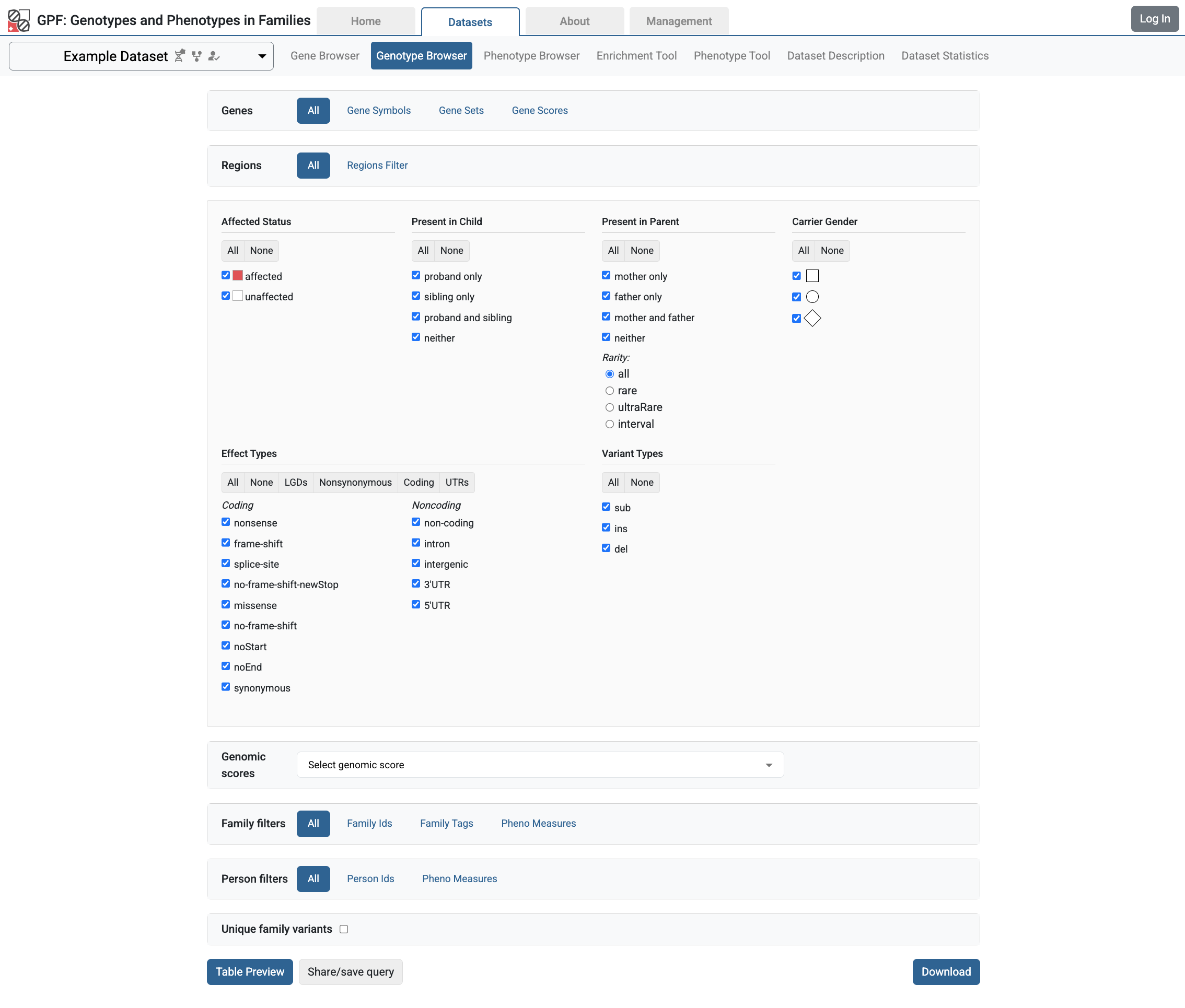
Now we can run the GPF development web server and browse our empty GPF instance:
wgpf run
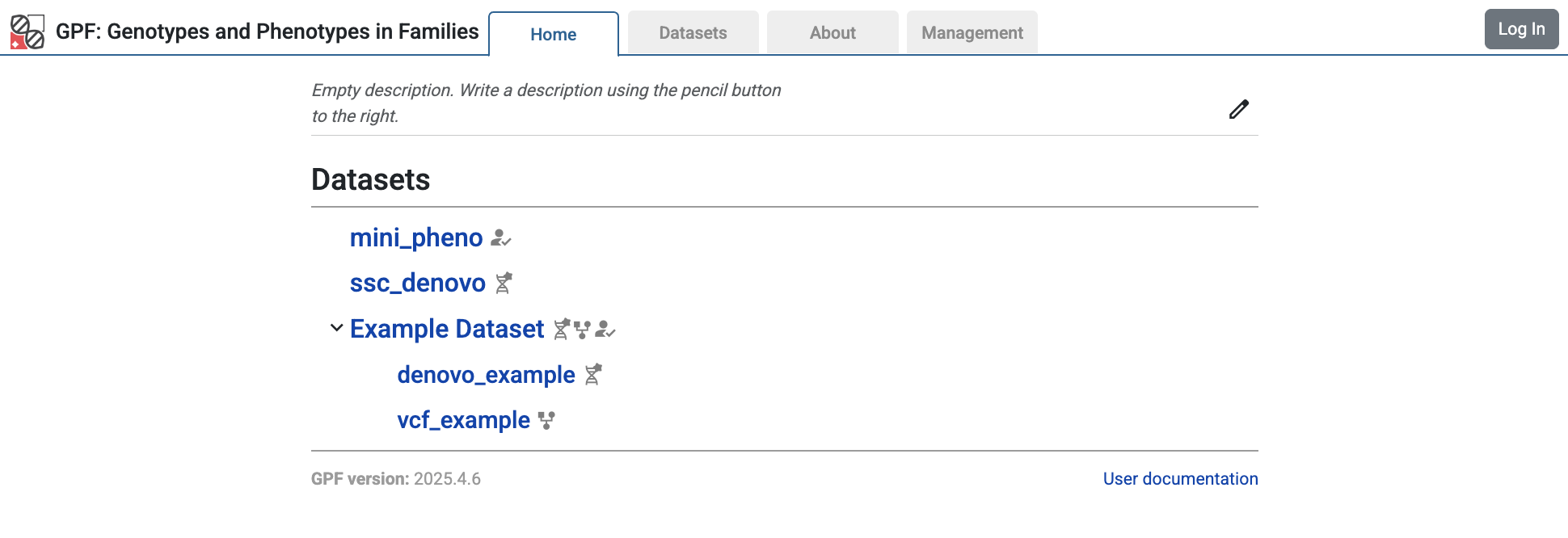
and browse the GPF development server at http://localhost:8000.
The web interface will be mostly empty as there is yet no data imported into the instance.
To stop the development GPF web server, you should press Ctrl-C - the usual
keybinding for stopping long-running commands in a terminal.
Warning
The development web server, run by wgpf run used in this guide, is
meant for development purposes only and is not suitable for serving the GPF
system in production.
Importing genotype data
Import Tools and Import Project
The tool used to import genotype data is named import_genotypes. This tool
expects an import project file that describes the import.
We support importing variants from multiple formats.
For this demonstration, we will be importing from the following formats:
List of de novo variants
Variant Call Format (VCF)
Example import of de novo variants
Let us import a small list of de novo variants.
Note
All the data files needed for this example are available in the
gpf-getting-started
repository under the subdirectory input_genotype_data.
A pedigree file that describes the families is needed -
input_genotype_data/example.ped:
We will also need the list of de novo variants
input_genotype_data/example.tsv:
A project configuration file for importing this study -
input_genotype_data/denovo_example.yaml - is also provided:
To import this project, run the following command:
import_genotypes input_genotype_data/denovo_example.yaml
Note
For more information on the import project configuration file, see Import Tools.
For more information on working with pedigree files, see Working With Pedigree Files Guide.
The import genotypes tool will read all the variants from the files
specified in the project configuration, annotate them using the reference
genome and gene models specified in the GPF instance configuration and finally
store them in an appropriate format for use by the GPF system. By default, the
imported files are stored in the internal_storage subdirectory of the GPF
instance directory.
A minimal study configuration file for the imported study will also be created
at minimal_instance/studies/denovo_example.yaml.
Intermediary files created during import will be stored in the import project
directory input_genotype_data/denovo_example.
When the import finishes, you can run the GPF development server using:
wgpf run
and browse the content of the GPF development server at
http://localhost:8000
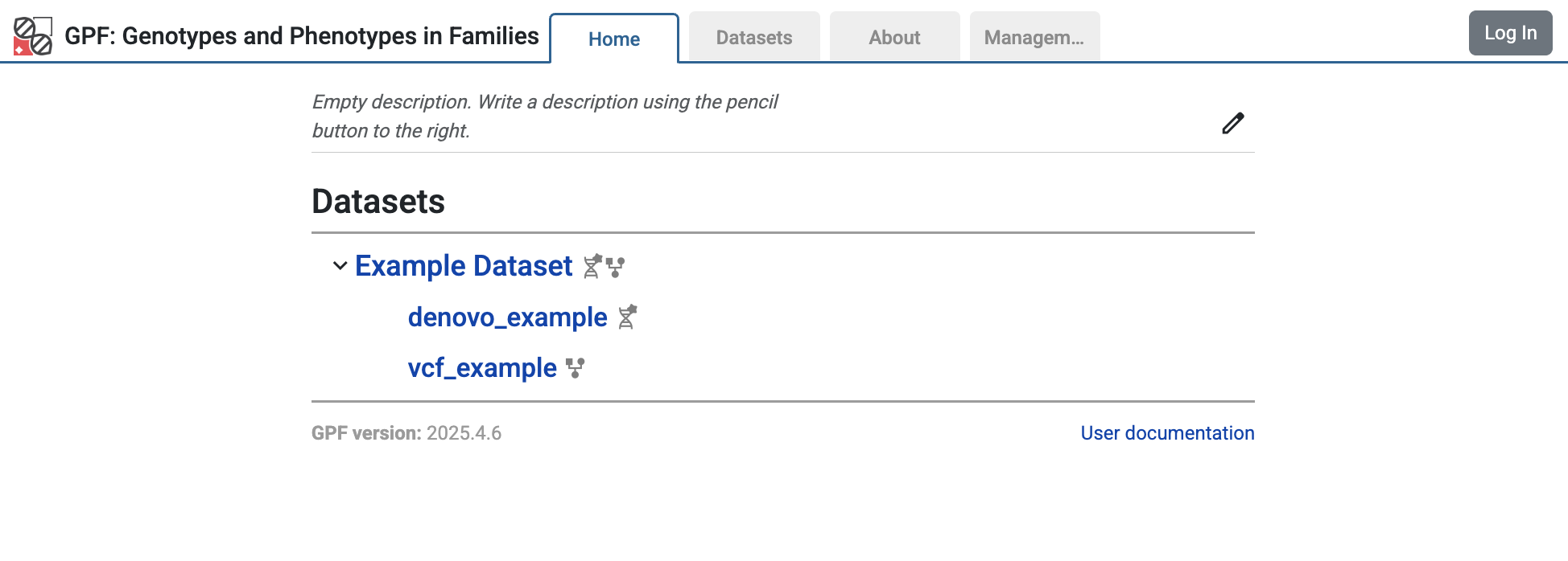
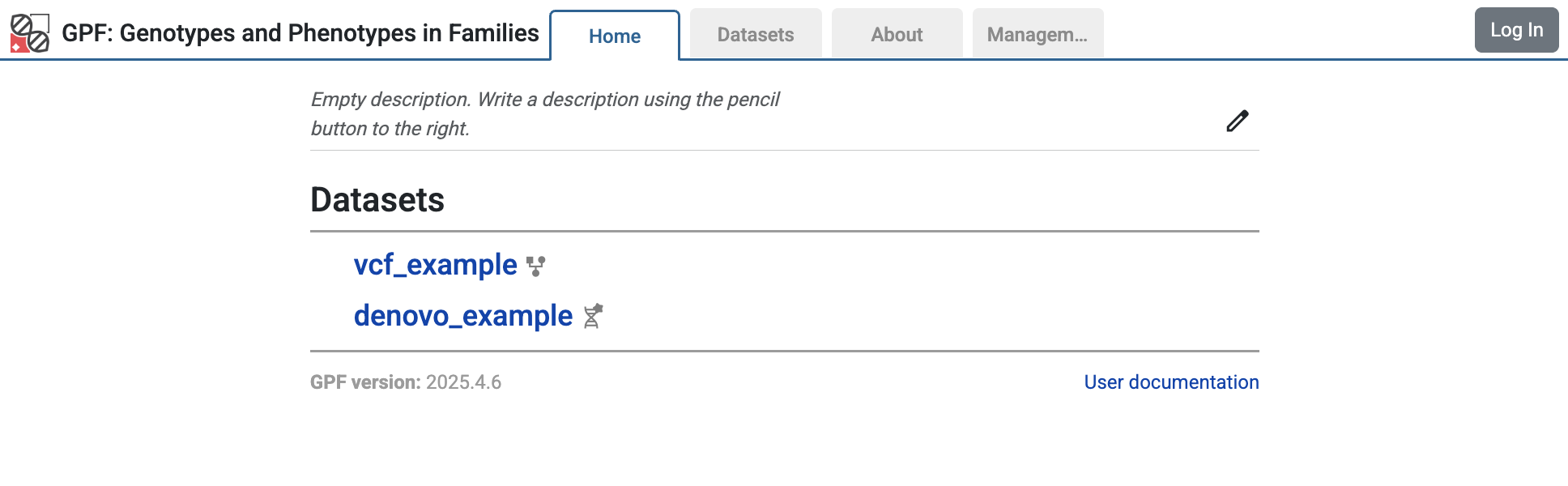
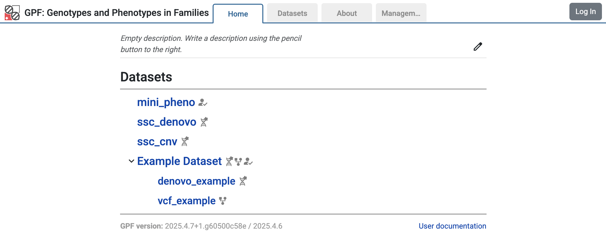
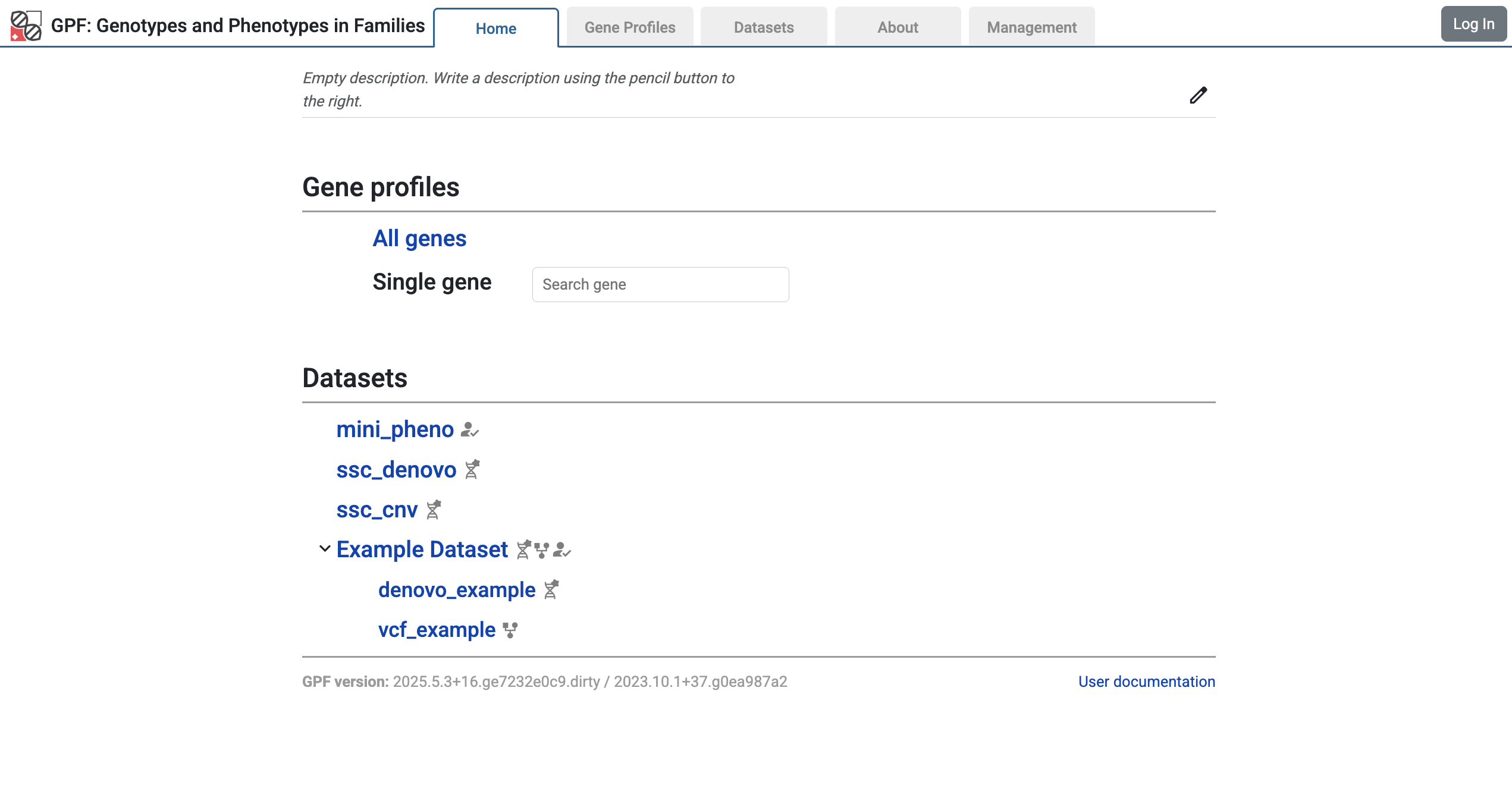
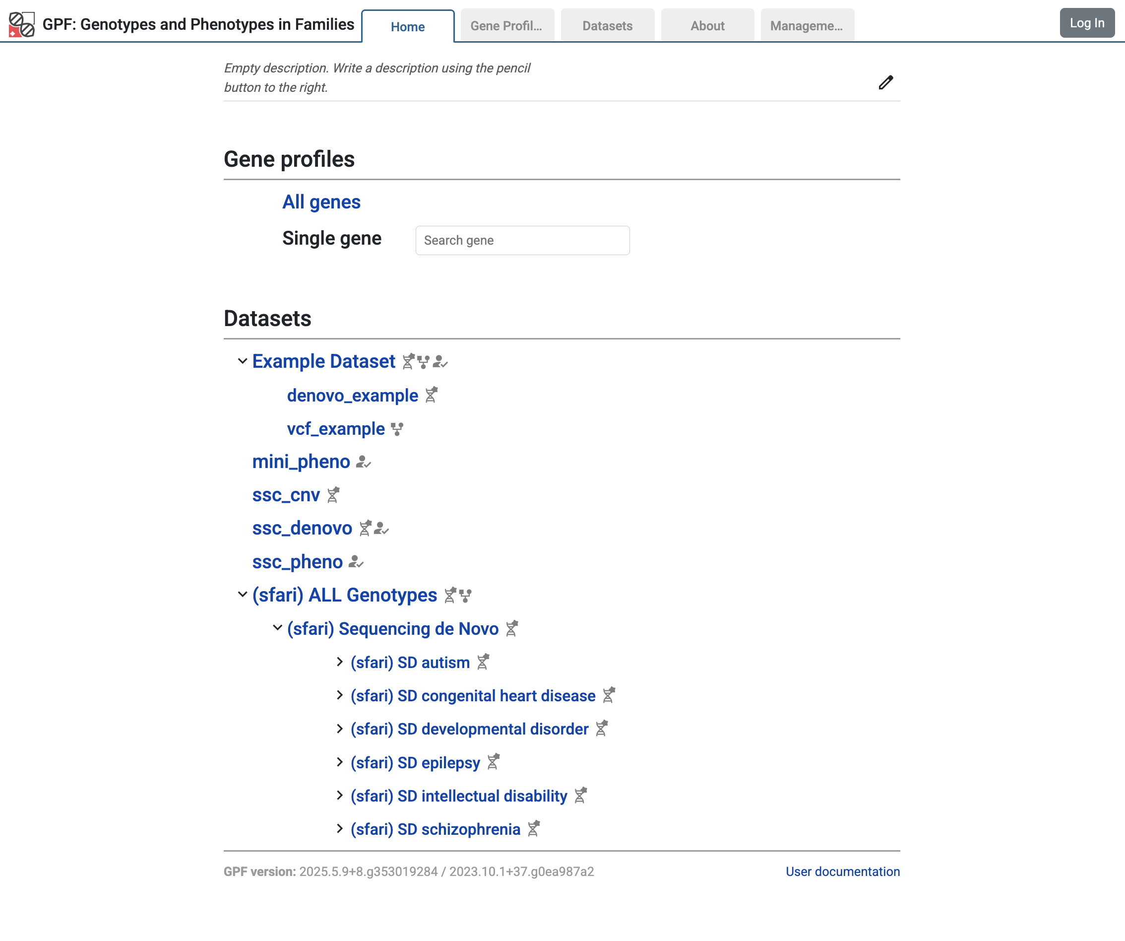
The home page of the GPF system will show the imported study
denovo_example.
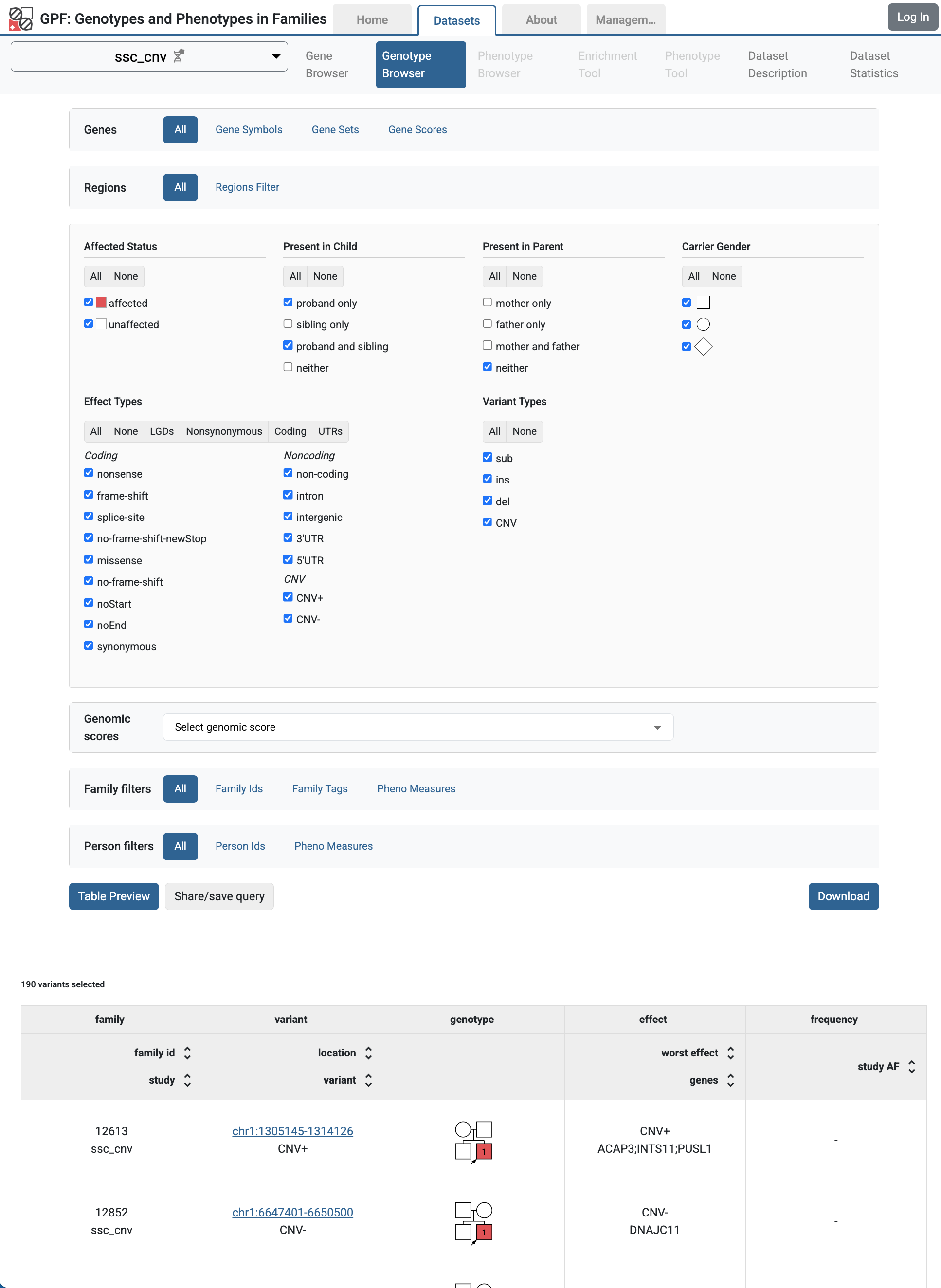
If you follow the link to the study and choose the Dataset Statistics page, you will see some summary information for the imported study: families and individuals included in the study, types of families, and rates of de novo variants.
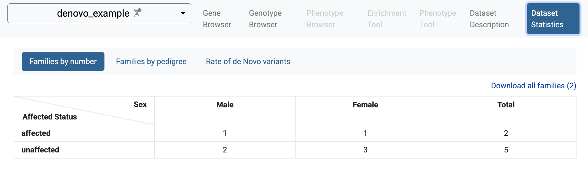
Statistics of individuals by affected status and sex
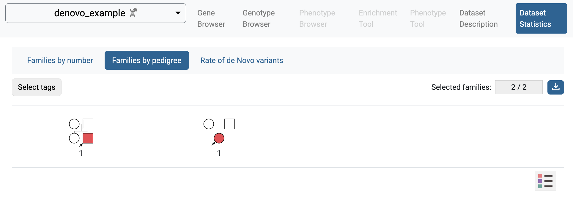
Statistics of families by family type
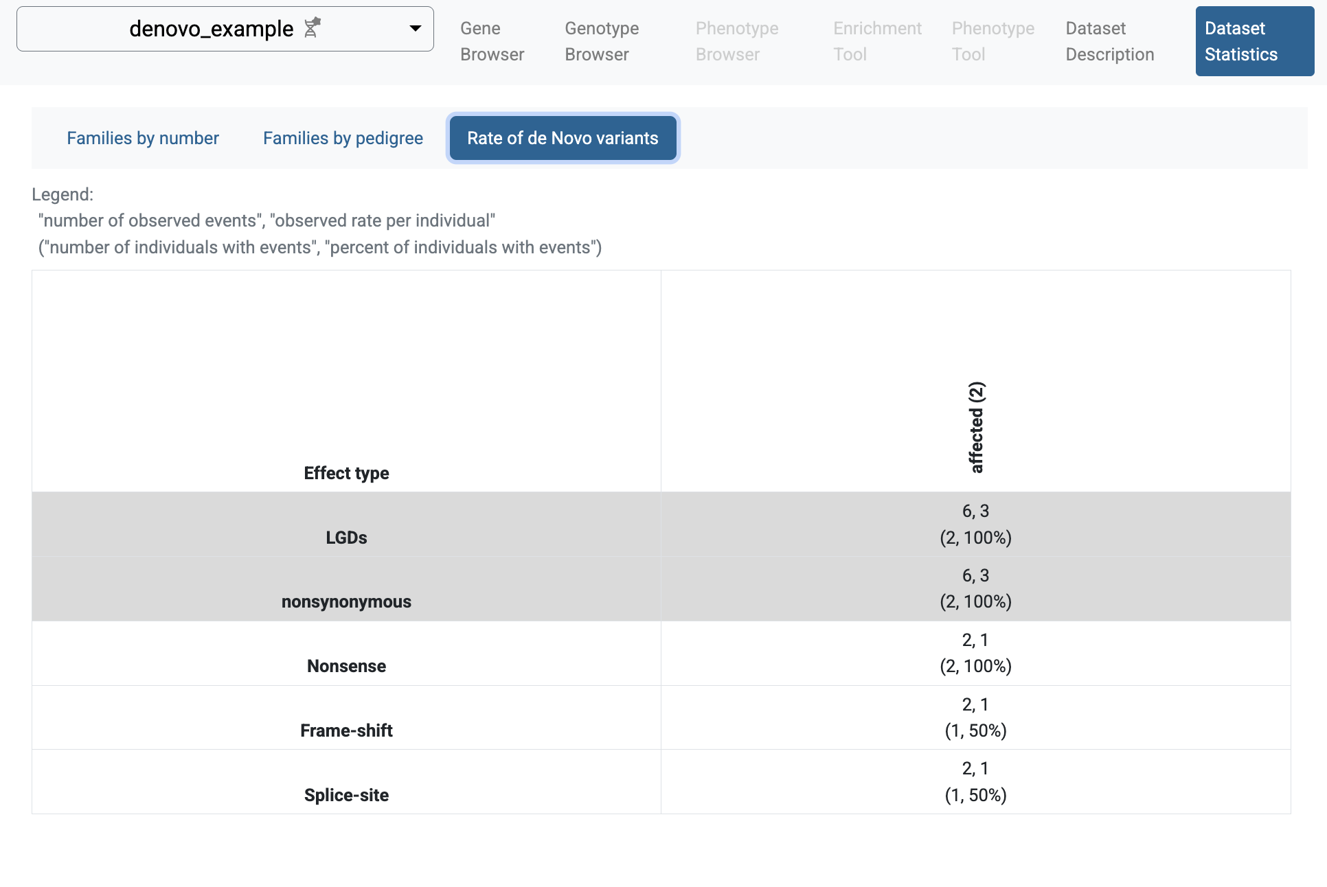
Rate of de novo variants
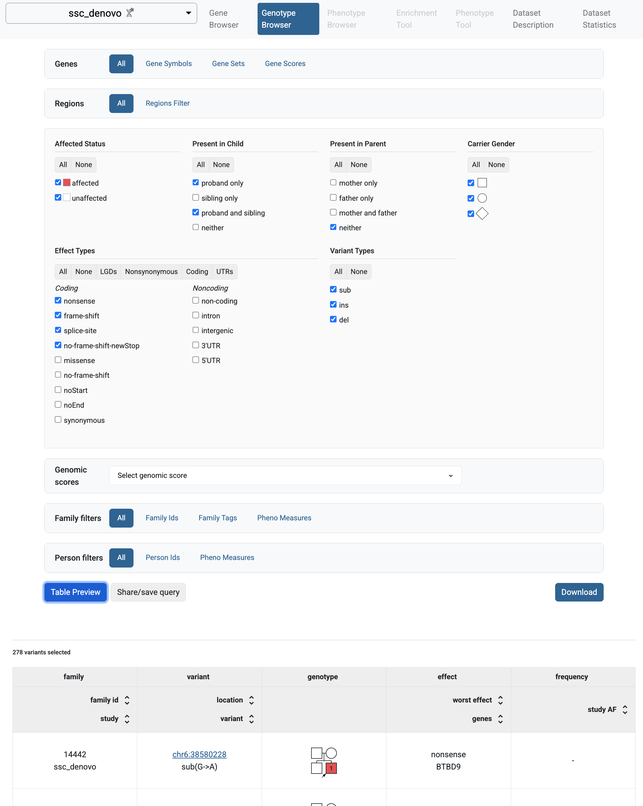
If you select the Genotype Browser page, you will be able to see the imported de novo variants. The default filters search for LGD de novo variants. It happens that all de novo variants imported in the denovo_example study are LGD variants.
So, when you click the Table Preview button, all the imported variants will be shown.
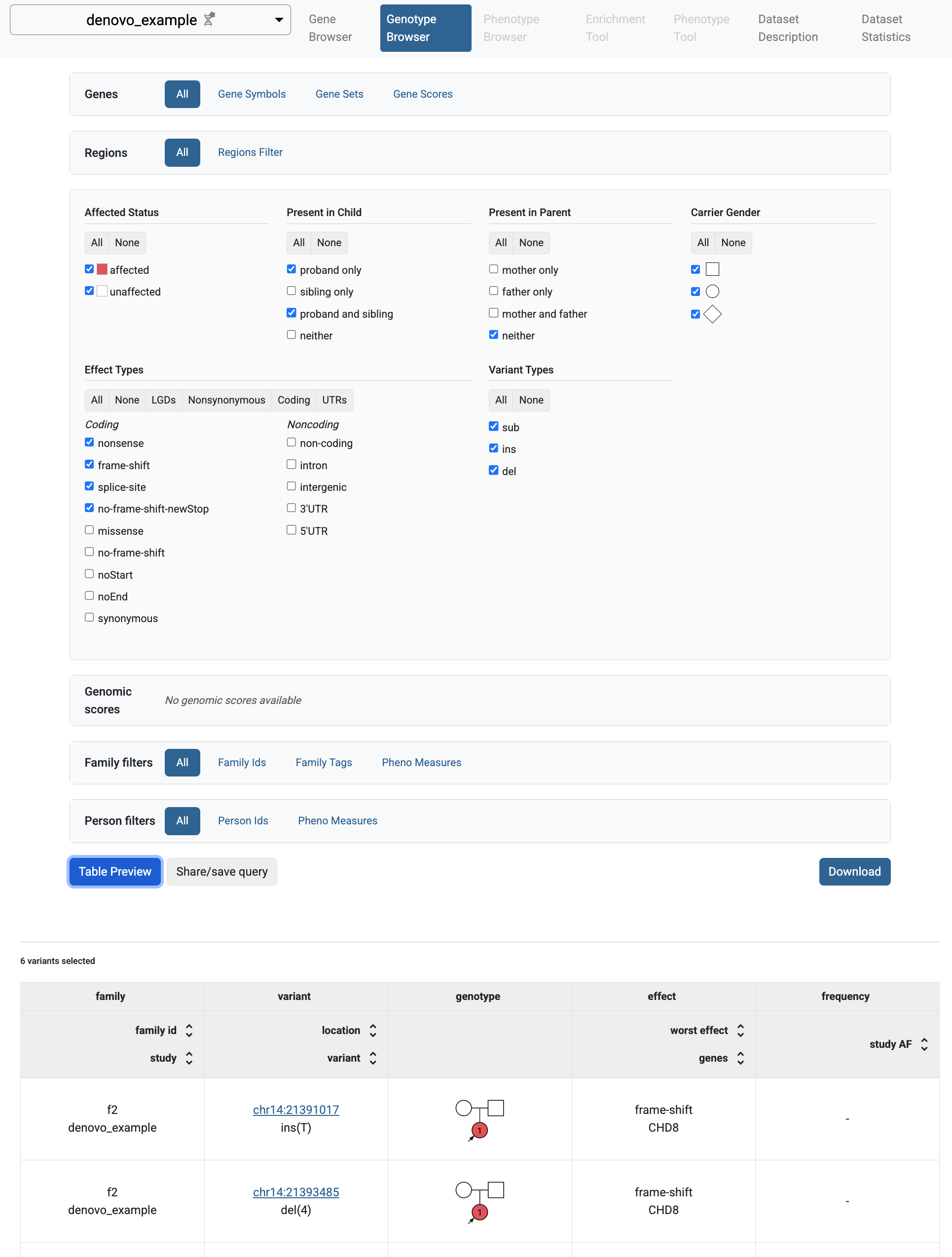
Genotype Browser with de novo variants
Example import of VCF variants
Similar to the sample denovo variants, there are also sample variants in
VCF format. They can be found in input_genotype_data/example.vcf;
the same pedigree file from before is used.
A project configuration file is provided -
input_genotype_data/vcf_example.yaml.
To import them, run the following command:
import_genotypes input_genotype_data/vcf_example.yaml
When the import finishes, you can run the GPF development server using:
wgpf run
and browse the content of the GPF development server at
http://localhost:8000
The GPF instance Home Page now includes the imported study vcf_example.
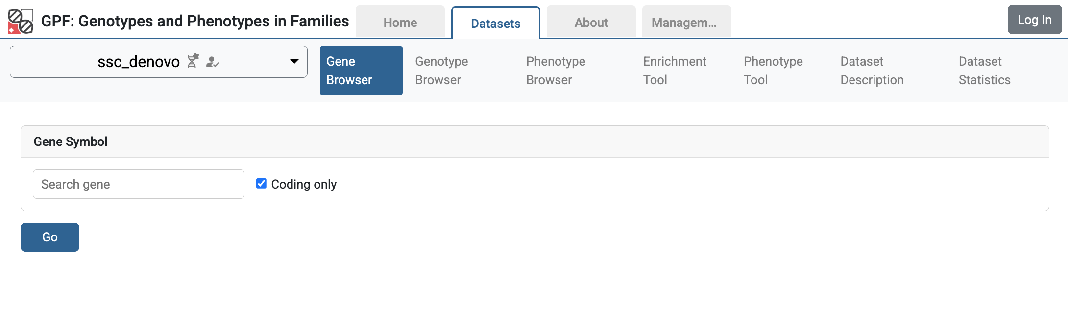
If you follow the link to the vcf_example, you will get to the Gene Browser page for the study. It happens that all imported VCF variants are located on the CHD8 gene. Fill CHD8 in the Gene Symbol box and click the Go button.
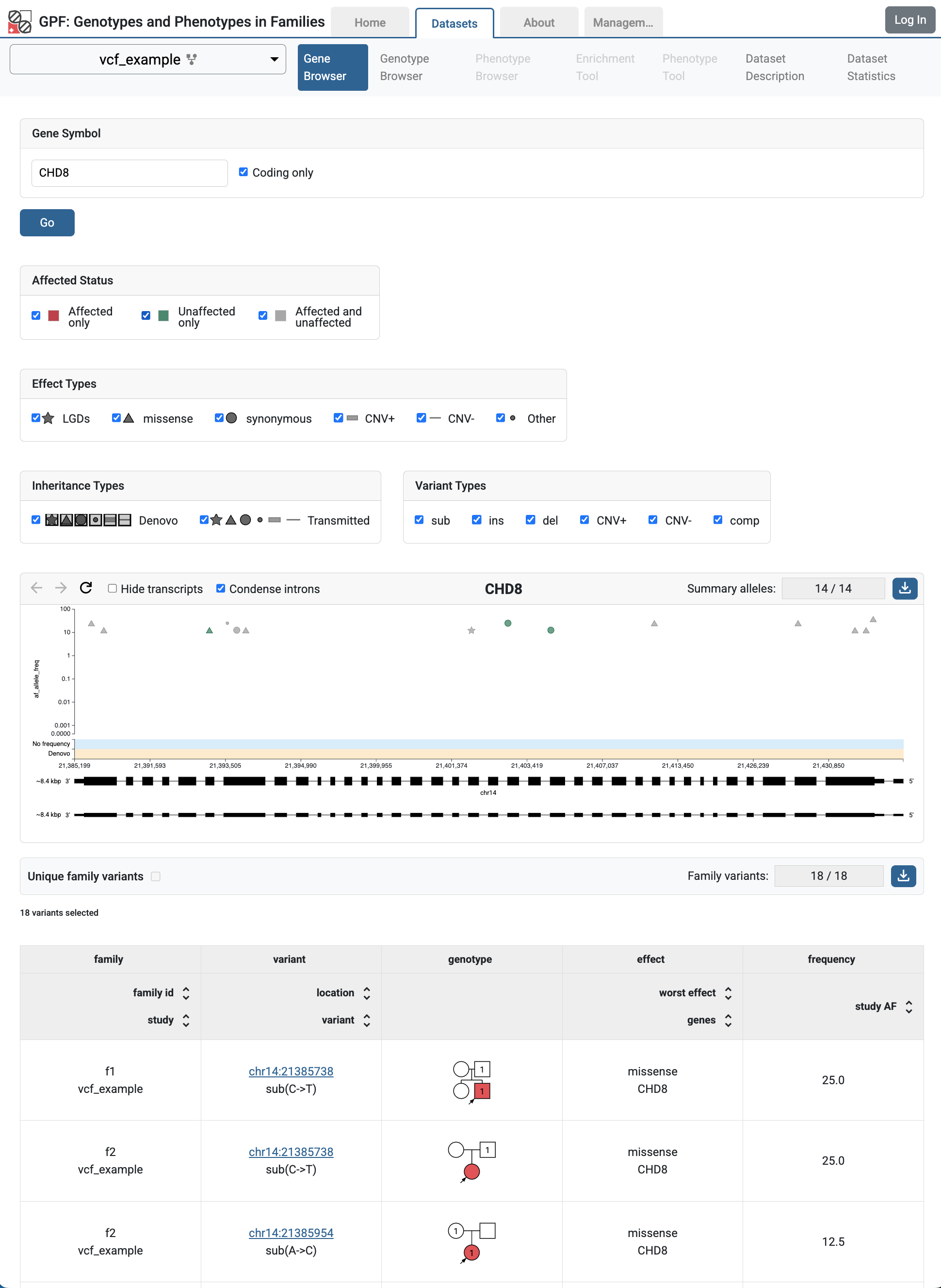
Gene Browser` for CHD8 gene shows variants from vcf_example study
In Gene Browser results, the top section has the summary variants, which show the location and frequency of the variants, the bottom section has the family variants, which show the family information, pedigree, and additional annotations.
The user may also observe these variants in the genotype browser by choosing:
‘All’ in Present in Child
‘All’ in Present in Parent and ‘all’ in Rarity
‘All’ in Effect Types.
Example of a dataset (group of genotype studies)
The already imported studies denovo_example and vcf_example
have genomic variants for the same group of individuals example.ped.
We can create a dataset (group of genotype studies) that includes both studies.
To this end, create a directory datasets/example_dataset inside the GPF
instance directory minimal_instance:
mkdir -p minimal_instance/datasets/example_dataset
and create the following configuration file example_dataset.yaml inside
that directory:
id: example_dataset
name: Example Dataset

studies:
  - denovo_example
  - vcf_example
When the configuration is ready, re-run the wgpf run command. The home page
of the GPF instance will change and now will include the configured dataset
example_dataset.

Home page of the GPF instance showing the example_dataset
Follow the link to the Example Dataset, choose the Gene Browser page, and fill in CHD8 in the Gene Symbol. Click the Go button, and now you will be able to see the variants from both studies.
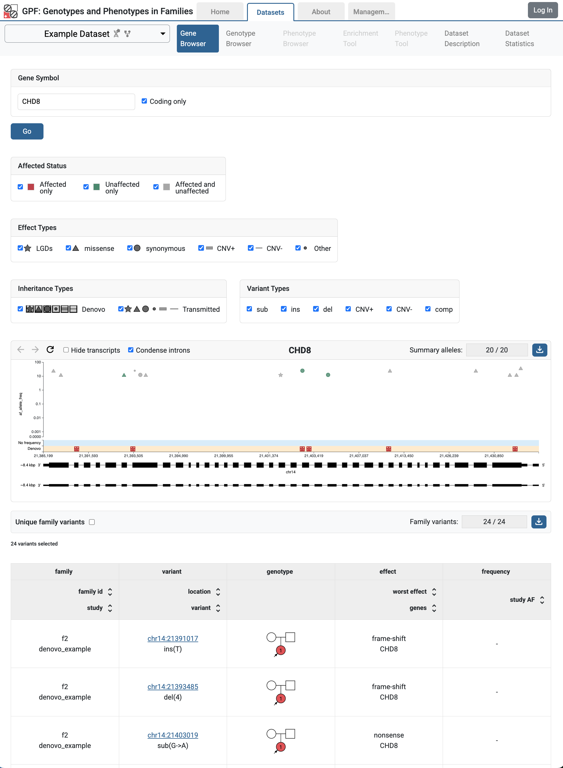
Gene Browser for CHD8 gene shows variants from both studies -
denovo_example and vcf_example
Getting Started with Annotation
The import of genotype data into a GPF instance always runs the GPF effect annotator. It is easy to extend the annotation of genotype data during the import.
To define the annotation used during the import into a GPF instance, we have to add a configuration that defines the pipeline of annotators and resources to be used during the import.
In the public GPF Genomic Resources Repository (GRR) there is a collection of public genomic resources available for use with GPF system.
Let’s say that we want to annotate the genotype variants with GnomAD and ClinVar. We need to find the appropriate resources in the public GRR:
hg38/variant_frequencies/gnomAD_4.1.0/genomes/ALL- this is anallele_scoreresource and the annotator by default produces one additional attributegnomad_v4_genome_ALL_afthat is the allele frequency for the variant (check the hg38/variant_frequencies/gnomAD_4.1.0/genomes/ALL page for more information about the resource);hg38/scores/ClinVar_20240730- this is anallele_scoreresource and the annotator by default produces two additional attributeCLNSIGthat is the aggregate germline classification for the variant andCLNDNthat is the preferred disease name (check the hg38/scores/ClinVar_20240730 page for more information about the resource.
In order to use these resources in the GPF instance annotation, we need to
edit the GPF instance configuration (minimal_instance/gpf_instance.yaml)
and add lines 9-12 to it:
 1instance_id: minimal_instance
 2
 3reference_genome:
 4  resource_id: "hg38/genomes/GRCh38-hg38"
 5
 6gene_models:
 7  resource_id: "hg38/gene_models/MANE/1.3"
 8
 9annotation:
10  config:
11    - allele_score: hg38/variant_frequencies/gnomAD_4.1.0/genomes/ALL
12    - allele_score: hg38/scores/ClinVar_20240730
When you start the GPF instance using the wgpf tool, it will automatically
re-annotate any genotype data that is not up to date:
wgpf run
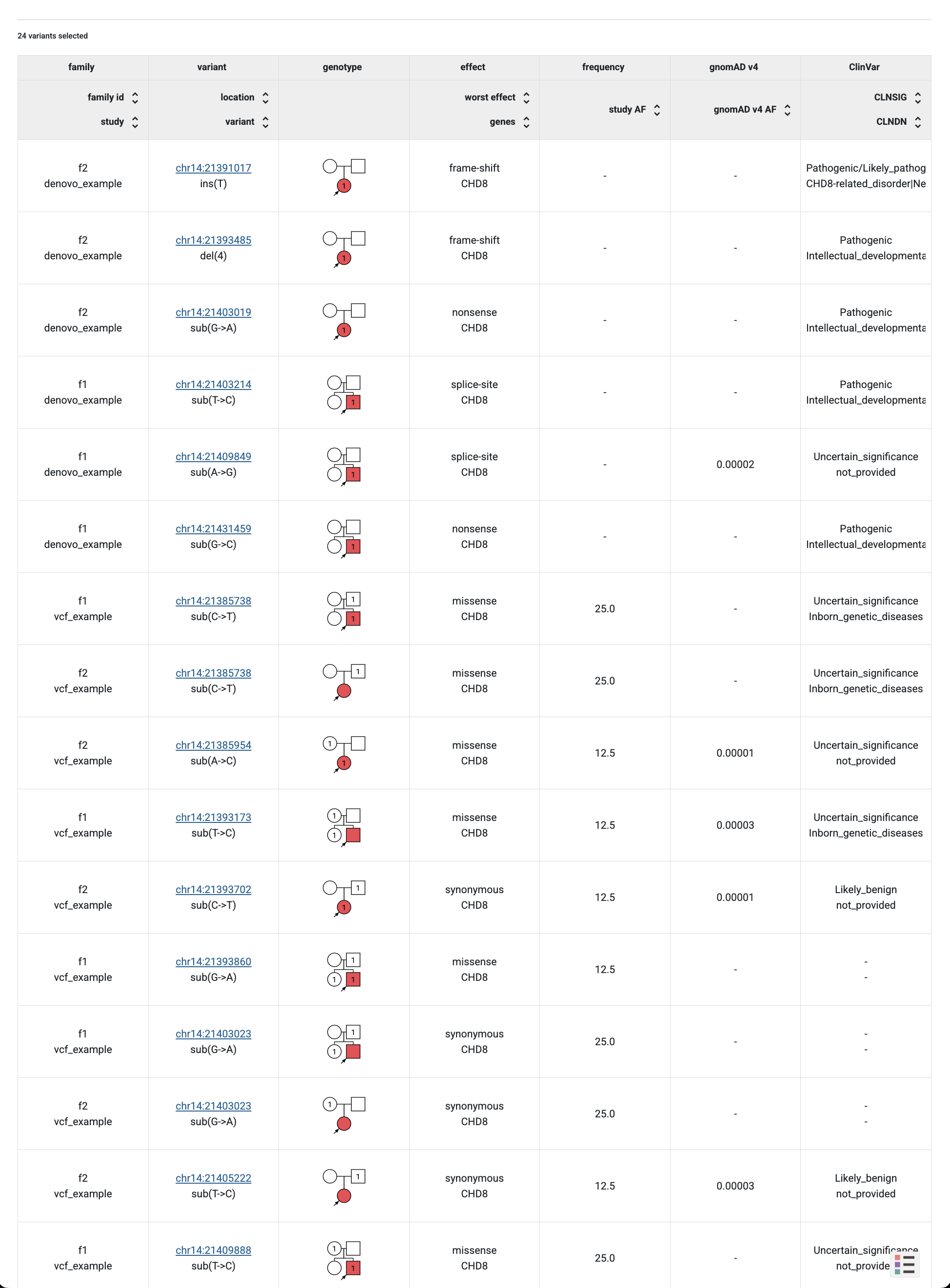
The variants in our Example Dataset will now have additional attributes that come from the annotation with GnomAD and ClinVar:
gnomad_v4_genome_ALL_afCLNSIGCLNDN
By default, the additional attributes produced by the annotation are usable in the following ways:
If you download the variants using the Genotype Browser download button, the additional attributes will be included in the downloaded file.
We can query the variants using the
gnomad_v4_genome_ALL_af,CLNSIGandCLNDNgenomic scores.
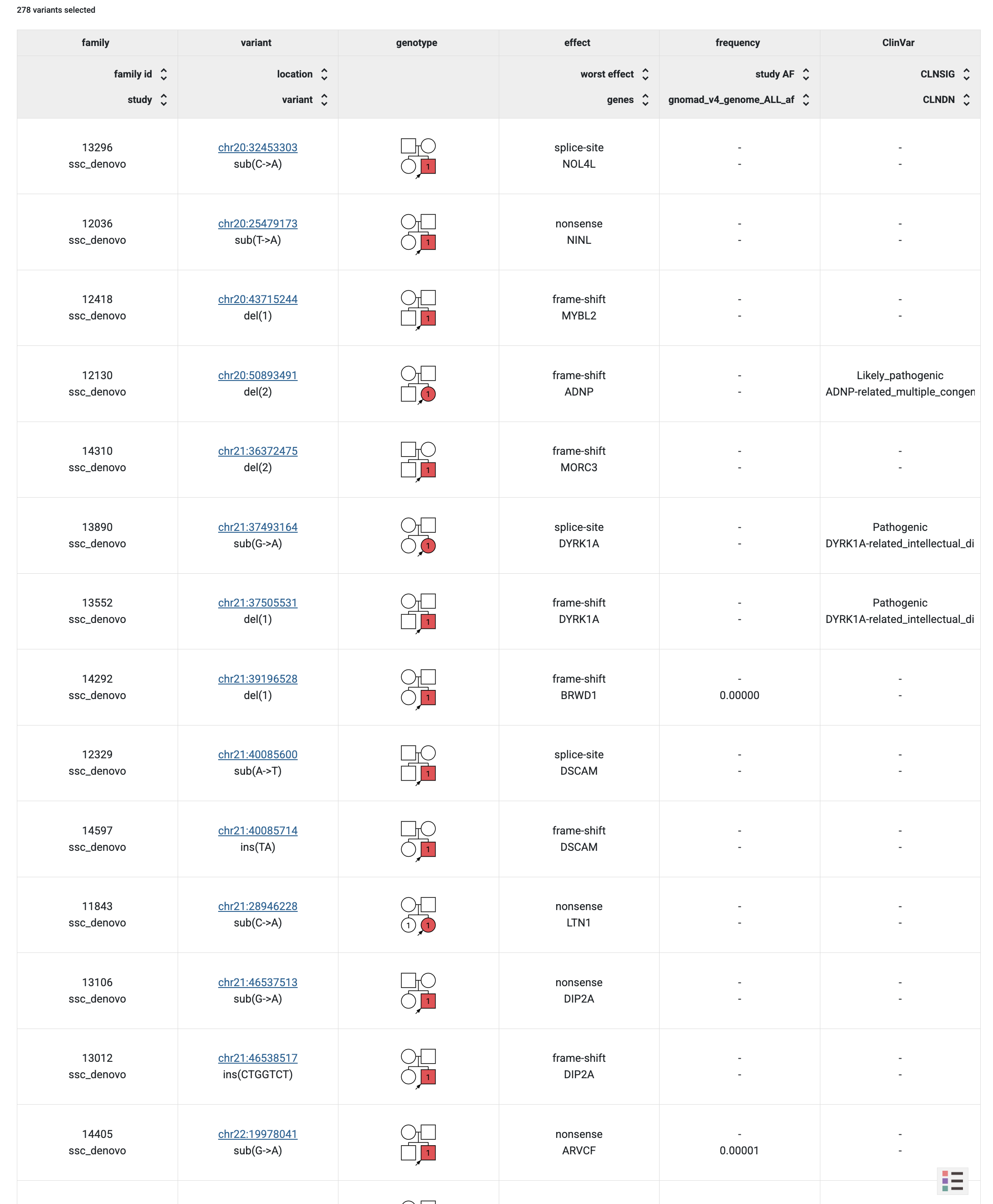
Let’s say we want to find all variants from Example Dataset that have gnomAD frequency. Navigate to the Genotype Browser tab for the Example Dataset. Select all checkboxes in the Genotype Browser filters. From the Genomic Score filter selects the gnomad_v4_genome_ALL_af score.
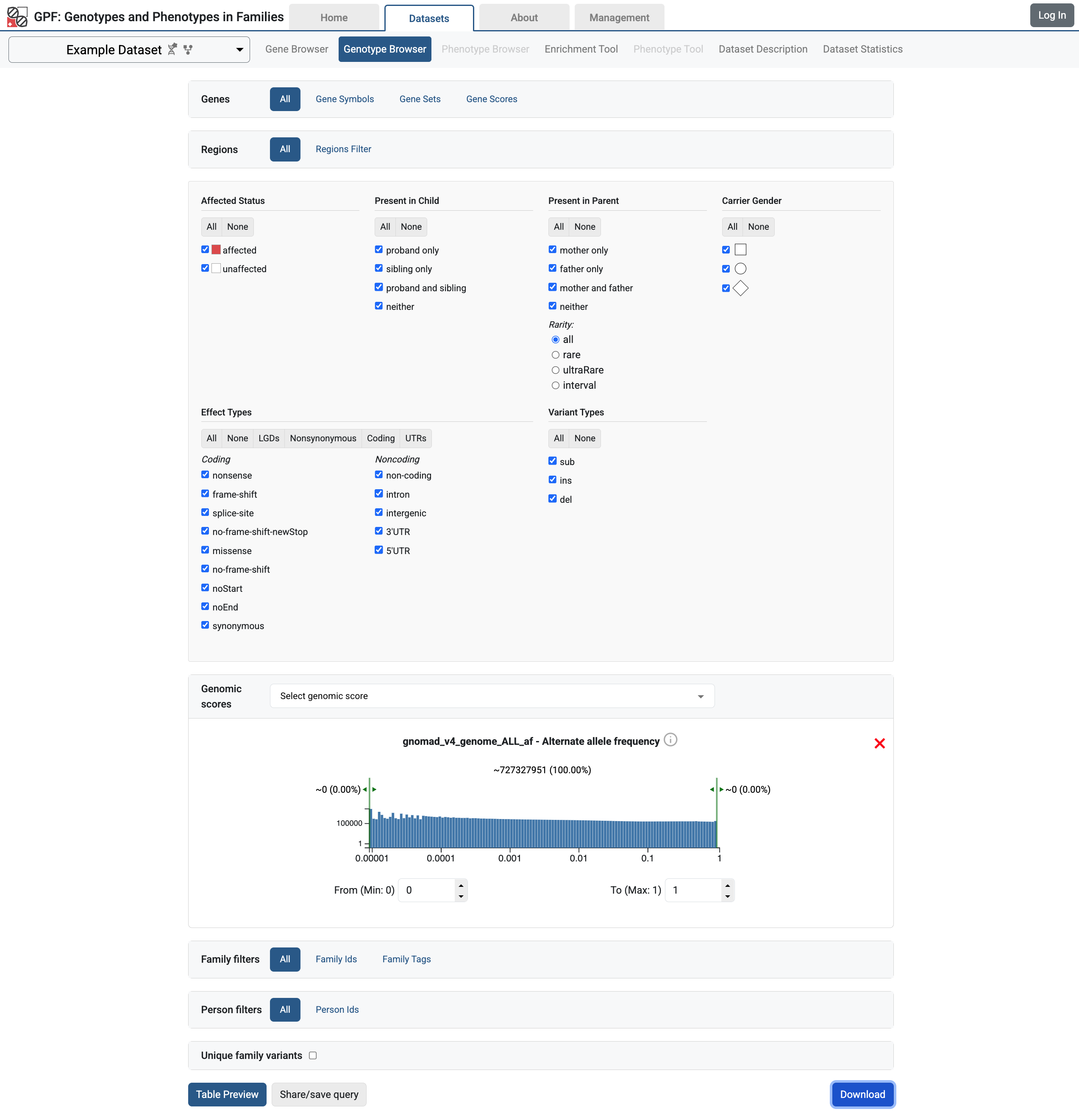
Genotype browser for Example Dataset with all filters selected
Then click on the Download button. This will download family variants matching the selected filters in a tab-separated file similar to the one shown bellow. Attributes from the annotation are included as the last columns in the downloaded file.
family id |
study |
location |
variant |
CHROM |
POS |
REF |
ALT |
family person ids |
family structure |
family best state |
family genotype |
carrier person ids |
carrier person attributes |
inheritance type |
family phenotypes |
carrier phenotypes |
parents called |
study AF |
worst effect |
genes |
all effects |
effect details |
gnomad_v4_genome_ALL_af |
CLNSIG |
CLNDN |
|---|---|---|---|---|---|---|---|---|---|---|---|---|---|---|---|---|---|---|---|---|---|---|---|---|---|
f1 |
denovo_example |
chr14:21409849 |
sub(A->G) |
chr14 |
21409849 |
A |
G |
f1.dad;f1.mom;f1.p1;f1.s1 |
dad:M:unaffected;mom:F:unaffected;prb:M:affected;sib:F:unaffected |
2212/0010 |
0/0;0/0;0/1;0/0 |
f1.p1 |
prb:M:affected |
denovo |
splice-site |
CHD8 |
CHD8:splice-site |
ENST00000646647.2:CHD8:splice-site:789/2581 |
0.00002 |
Uncertain_significance |
not_provided |
||||
f2 |
vcf_example |
chr14:21385954 |
sub(A->C) |
chr14 |
21385954 |
A |
C |
f2.mom;f2.dad;f2.p1 |
mom:F:unaffected;dad:M:unaffected;prb:F:affected |
121/101 |
0/1;0/0;0/1 |
f2.mom;f2.p1 |
mom:F:unaffected;prb:F:affected |
mendelian |
4 |
12.5 |
missense |
CHD8 |
CHD8:missense |
ENST00000646647.2:CHD8:missense:2469/2581(Ser->Ala) |
0.00001 |
Uncertain_significance |
not_provided |
||
f1 |
vcf_example |
chr14:21393173 |
sub(T->C) |
chr14 |
21393173 |
T |
C |
f1.dad;f1.mom;f1.p1;f1.s1 |
dad:M:unaffected;mom:F:unaffected;prb:M:affected;sib:F:unaffected |
2121/0101 |
0/0;0/1;0/0;0/1 |
f1.mom;f1.s1 |
mom:F:unaffected;sib:F:unaffected |
mendelian |
4 |
12.5 |
missense |
CHD8 |
CHD8:missense |
ENST00000646647.2:CHD8:missense:2134/2581(Asp->Gly) |
0.00003 |
Uncertain_significance |
Inborn_genetic_diseases |
||
f2 |
vcf_example |
chr14:21393702 |
sub(C->T) |
chr14 |
21393702 |
C |
T |
f2.mom;f2.dad;f2.p1 |
mom:F:unaffected;dad:M:unaffected;prb:F:affected |
211/011 |
0/0;0/1;0/1 |
f2.dad;f2.p1 |
dad:M:unaffected;prb:F:affected |
mendelian |
4 |
12.5 |
synonymous |
CHD8 |
CHD8:synonymous |
ENST00000646647.2:CHD8:synonymous:2031/2581 |
0.00001 |
Likely_benign |
not_provided |
||
f2 |
vcf_example |
chr14:21405222 |
sub(T->C) |
chr14 |
21405222 |
T |
C |
f2.mom;f2.dad;f2.p1 |
mom:F:unaffected;dad:M:unaffected;prb:F:affected |
212/010 |
0/0;0/1;0/0 |
f2.dad |
dad:M:unaffected |
mendelian |
4 |
12.5 |
synonymous |
CHD8 |
CHD8:synonymous |
ENST00000646647.2:CHD8:synonymous:1098/2581 |
0.00003 |
Likely_benign |
not_provided |
||
f1 |
vcf_example |
chr14:21431306 |
sub(G->A) |
chr14 |
21431306 |
G |
A |
f1.dad;f1.mom;f1.p1;f1.s1 |
dad:M:unaffected;mom:F:unaffected;prb:M:affected;sib:F:unaffected |
1211/1011 |
0/1;0/0;0/1;0/1 |
f1.dad;f1.p1;f1.s1 |
dad:M:unaffected;prb:M:affected;sib:F:unaffected |
mendelian |
4 |
12.5 |
missense |
CHD8 |
CHD8:missense |
ENST00000646647.2:CHD8:missense:113/2581(Ser->Leu) |
0.00005 |
Conflicting_classifications_of_pathogenicity |
Inborn_genetic_diseases|not_provided |
||
f2 |
vcf_example |
chr14:21431623 |
sub(A->C) |
chr14 |
21431623 |
A |
C |
f2.mom;f2.dad;f2.p1 |
mom:F:unaffected;dad:M:unaffected;prb:F:affected |
100/122 |
0/1;1/1;1/1 |
f2.mom;f2.dad;f2.p1 |
mom:F:unaffected;dad:M:unaffected;prb:F:affected |
mendelian |
4 |
37.5 |
missense |
CHD8 |
CHD8:missense |
ENST00000646647.2:CHD8:missense:7/2581(Asp->Glu) |
0.00001 |
Uncertain_significance |
not_provided|Inborn_genetic_diseases |
||
f1 |
vcf_example |
chr14:21393541 |
del(3) |
chr14 |
21393540 |
GGAA |
G |
f1.dad;f1.mom;f1.p1;f1.s1 |
dad:M:unaffected;mom:F:unaffected;prb:M:affected;sib:F:unaffected |
1102/1120 |
0/1;0/1;1/1;0/0 |
f1.dad;f1.mom;f1.p1 |
dad:M:unaffected;mom:F:unaffected;prb:M:affected |
mendelian |
4 |
25.0 |
no-frame-shift |
CHD8 |
CHD8:no-frame-shift |
ENST00000646647.2:CHD8:no-frame-shift:2084/2581(SerSer->Ser) |
0.00013 |
Conflicting_classifications_of_pathogenicity |
Intellectual_developmental_disorder_with_autism_and_macrocephaly|not_provided |
||
f2 |
vcf_example |
chr14:21431499 |
sub(T->C) |
chr14 |
21431499 |
T |
C |
f2.mom;f2.dad;f2.p1 |
mom:F:unaffected;dad:M:unaffected;prb:F:affected |
211/011 |
0/0;0/1;0/1 |
f2.dad;f2.p1 |
dad:M:unaffected;prb:F:affected |
mendelian |
4 |
12.5 |
missense |
CHD8 |
CHD8:missense |
ENST00000646647.2:CHD8:missense:49/2581(Met->Val) |
0.00276 |
Benign |
not_provided|Inborn_genetic_diseases |
Note
The attributes produced by the annotation can be used in the Genotype Browser preview table as described in Getting Started with Preview Columns.
Getting Started with Phenotype Data
Importing phenotype data
The import_phenotypes tool is used to import phenotype data.
Note
All the data files needed for this example are available in the
gpf-getting-started
repository under the subdirectory input_phenotype_data.
The tool requires an import project, a YAML file describing the contents of the phenotype data to be imported, along with configuration options on how to import them.
As an example, we are going to show how to import a simulated phenotype data into our GPF instance.
Inside the input_phenotype_data directory, the following data is provided:
pedigree.pedis the phenotype data pedigree file.input_phenotype_data/pedigree.ped:instrumentscontains the phenotype instruments and measures to be imported. There are two instruments in the example:measure_descriptions.tsvcontains descriptions of the provided measures.input_phenotype_data/measure_descriptions.tsv:import_project.yamlis the import project configuration that we will use to import this data.input_phenotype_data/import_project.yaml:
Note
For more information on how to import phenotype data, see Phenotype Database Tools
We will use the import_phenotypes tool to import the phenotype data.
It will import the phenotype database directly to our GPF instance’s phenotype
storage:
import_phenotypes input_phenotype_data/import_project.yaml
When the import finishes, you can run the GPF development server using:
wgpf run
Now, on the GPF instance Home Page, you should see the mini_pheno
phenotype study.
Home page with imported phenotype study
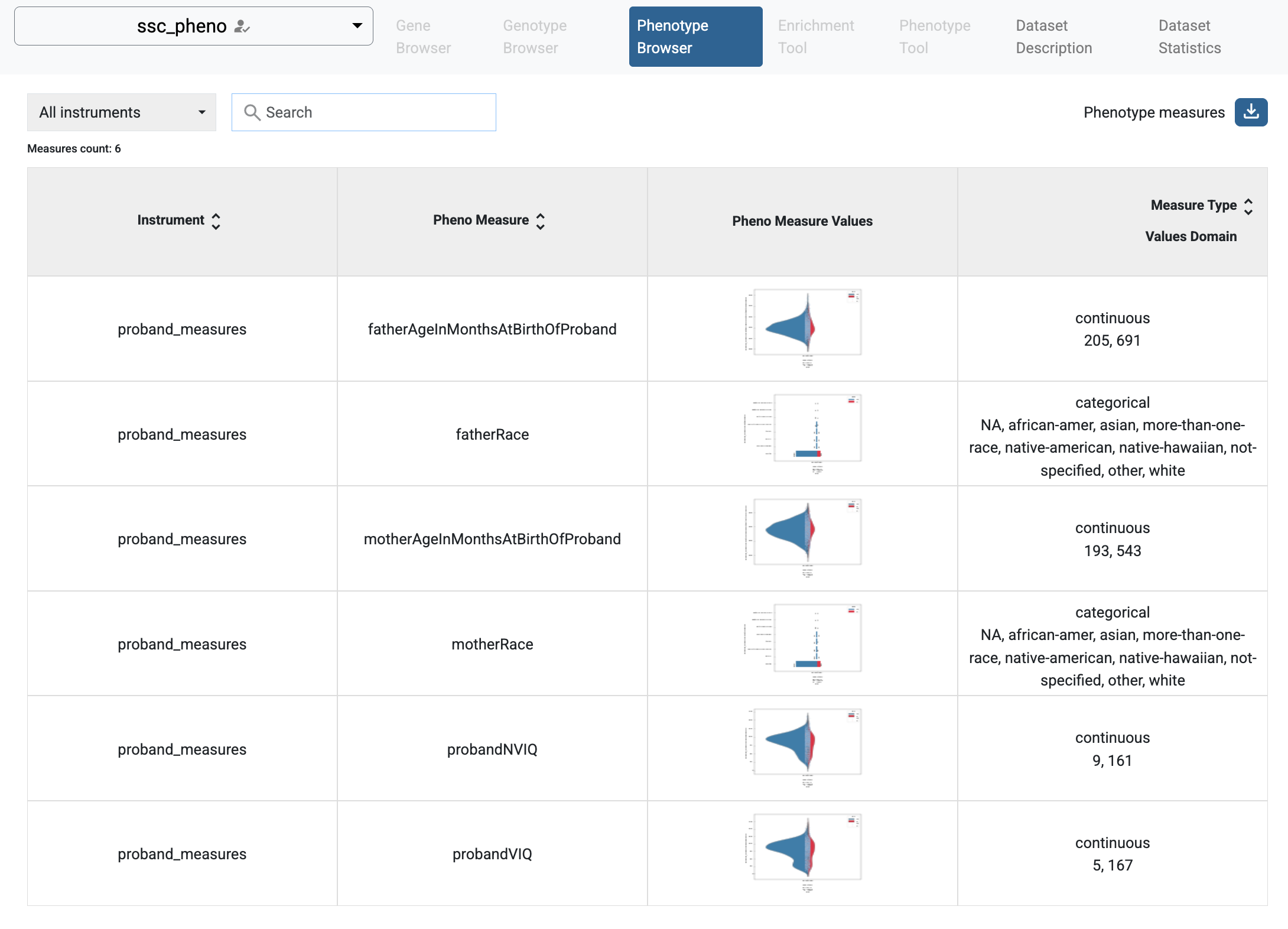
If you follow the link, you will see the Phenotype Browser tab with the imported data.
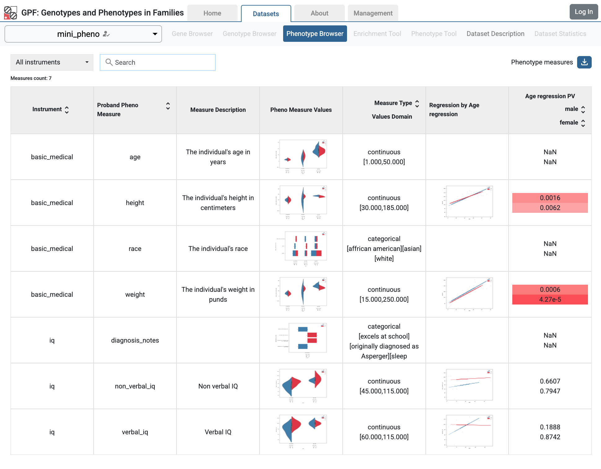
Phenotype Browser tab with imported data
In the Phenotype Browser tab, you can search for phenotype instruments and measures, see the aggregated figures for the measures, and download selected instruments and measures.
Configure a genotype study to use phenotype data
To demonstrate how a study is configured with a phenotype database, we will
be working with the already configured example_dataset dataset.
The phenotype databases can be attached to one or more studies and/or datasets.
If you want to attach the mini_pheno phenotype study to the
example_dataset dataset,
you need to specify it in the dataset’s configuration file, which can be found
at minimal_instance/datasets/example_dataset/example_dataset.yaml.
Add the following line to the configuration file:
phenotype_data: mini_pheno
When you restart the server, you should be able to see Phenotype Browser and Phenotype Tool tabs enabled for the Example Dataset dataset.
Additionally, in the Genotype Browser, the Family Filters and Person Filters sections will have the Pheno Measures filters enabled.
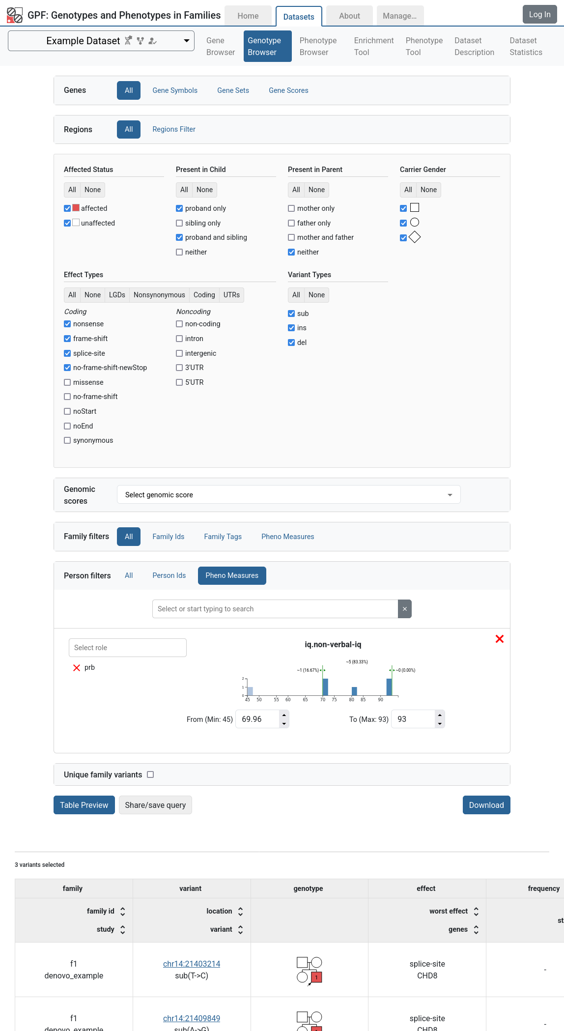
Example Dataset genotype browser using Pheno Measures family filters
Getting Started with Preview Columns
Configure genotype columns in Genotype Browser
Once you have annotated your variants, the additional attributes produced by the annotation can be displayed in the variants preview table.
In our example, the annotation produces three additional attributes:
gnomad_v4_genome_ALL_afCLNSIGCLNDN
Let us add these attributes to the variants preview table for the
example_dataset dataset.
In the preview table, each column could show multiple values. In GPF, when you want to show multiple values in a single column, you need to define a column group.
The column group is a collection of attributes that are shown together in the preview table. The values in a column group are shown in a single cell.
By default, the study configuration includes several predefined column groups:
family, variant, genotype, effect and frequency.
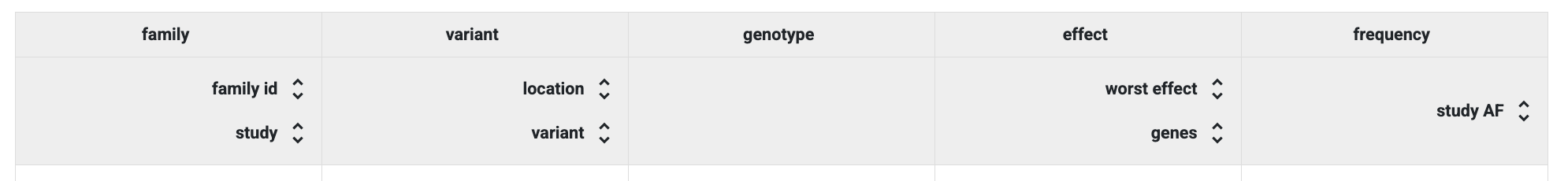
Default column groups in the Preview Table
In the study configuration, you can define new column groups or redefine
already existing ones. Let us redefine the existing column group
frequency to include the gnomAD frequency and define a new column group
clinvar to include the ClinVar attributes.
The column group is defined in the
column_groups section of the configuration file.
Edit the example_dataset.yaml dataset configuration in
minimal_instance/datasets/example_dataset and add the following section
at the end of the configuration file:
 1genotype_browser:
 2  column_groups:
 3    frequency:
 4      name: frequency
 5      columns:
 6      - allele_freq
 7      - gnomad_v4_genome_ALL_af
 8
 9    clinvar:
10      name: ClinVar
11      columns:
12      - CLNSIG
13      - CLNDN
14
15  preview_columns_ext:
16    - clinvar
In lines 3-7, we re-define the existing column group
frequency to include the study frequency allele_freq and gnomAD
frequency gnomad_v4_genome_ALL_af.
In lines 9-13, we define a new column group
clinvar that contains the values of the annotation attributes
CLNSIG and CLNDN.
In lines 15-16, we extend the preview table columns. The new column groups
clinvar will be added to the preview table.
If we now stop the wgpf tool and rerun it, we will be able to see
the new columns in the preview table.
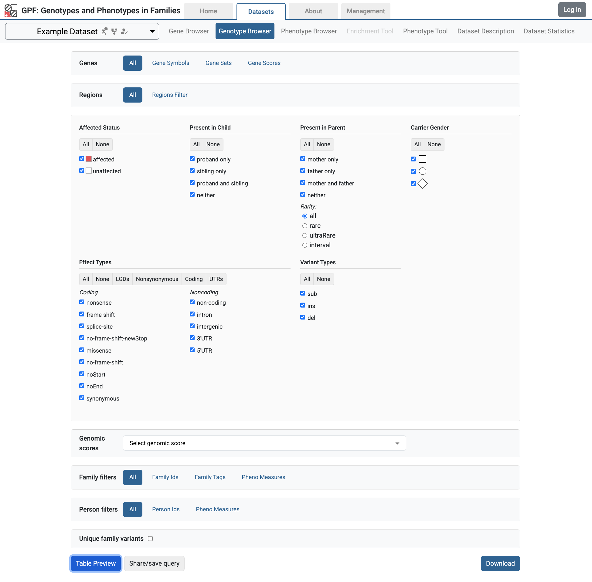
From the GPF instance Home Page, follow the link to the Example Dataset page and choose the Genotype Browser. Select all checkboxes in Present in Child, Present in Parent and Effect Types sections.
Then click the Preview button and will be able to see all the imported variants with their additional attributes coming from the annotation.
Example Dataset genotype browser displaying variants with additional columns gnomAD v4 and ClinVar.
Configure phenotype columns in Genotype Browser
The Genotype Browser allows you to add phenotype attributes to the table preview and the download file.
Phenotype attributes show values from a phenotype database that are associated with the displayed family variant. To configure such a column, you need to specify the following properties:
source- the measure ID whose values will be shown in the column;role- the role of the person in the family for which we are going to show the phenotype measure value;name- the display name of the column in the table.
Let’s add some phenotype columns to the Genotype Browser preview table
in Example Dataset.
To do this, you need to define them in the study’s config, in the genotype
browser section of the configuration file.
We are going to modify the
example_dataset.yaml dataset configuration in
minimal_instance/datasets/example_dataset/example_dataset.yaml:
 1genotype_browser:
 2  columns:
 3    phenotype:
 4      prb_verbal_iq:
 5        role: prb
 6        name: Verbal IQ
 7        source: iq.verbal_iq
 8
 9      prb_non_verbal_iq:
10        role: prb
11        name: Non-Verbal IQ
12        source: iq.non_verbal_iq
13
14  column_groups:
15    frequency:
16      name: frequency
17      columns:
18      - allele_freq
19      - gnomad_v4_genome_ALL_af
20
21    clinvar:
22      name: ClinVar
23      columns:
24      - CLNSIG
25      - CLNDN
26
27    proband_iq:
28      name: Proband IQ
29      columns:
30      - prb_verbal_iq
31      - prb_non_verbal_iq
32
33  preview_columns_ext:
34    - clinvar
35    - proband_iq
Lines 2-12 define the two new columns with values coming from the phenotype data attributes:
prb_verbal_iq- is a column that uses the value of the phenotype measureiq.verbal_iqfor the family proband. The display name of the column will be Verbal IQ;prb_non_verbal_iq- is a column that uses the value of the phenotype measureiq.non_verbal_iqfor the family proband. The display name of the column will be Non-Verbal IQ.
We want these two columns to be shown together in the preview table. To do
this, we need to define a new column group.
In lines 27-31, we define a column group called proband_iq that contains
the columns prb_verbal_iq and prb_non_verbal_iq.
To add the new column group proband_iq to the preview table, we need to
add it to the preview_columns_ext section of the configuration file.
In line 35, we add the new column group proband_iq at the end of the
preview table.
When you restart the server, go to the Genotype Browser tab of the
Example Dataset dataset and select all checkboxes in Present in Child,
Present in Parent and Effect Types sections:
When you click on the Table Preview button, you will be able to see the new
column group proband_iq in the preview table.
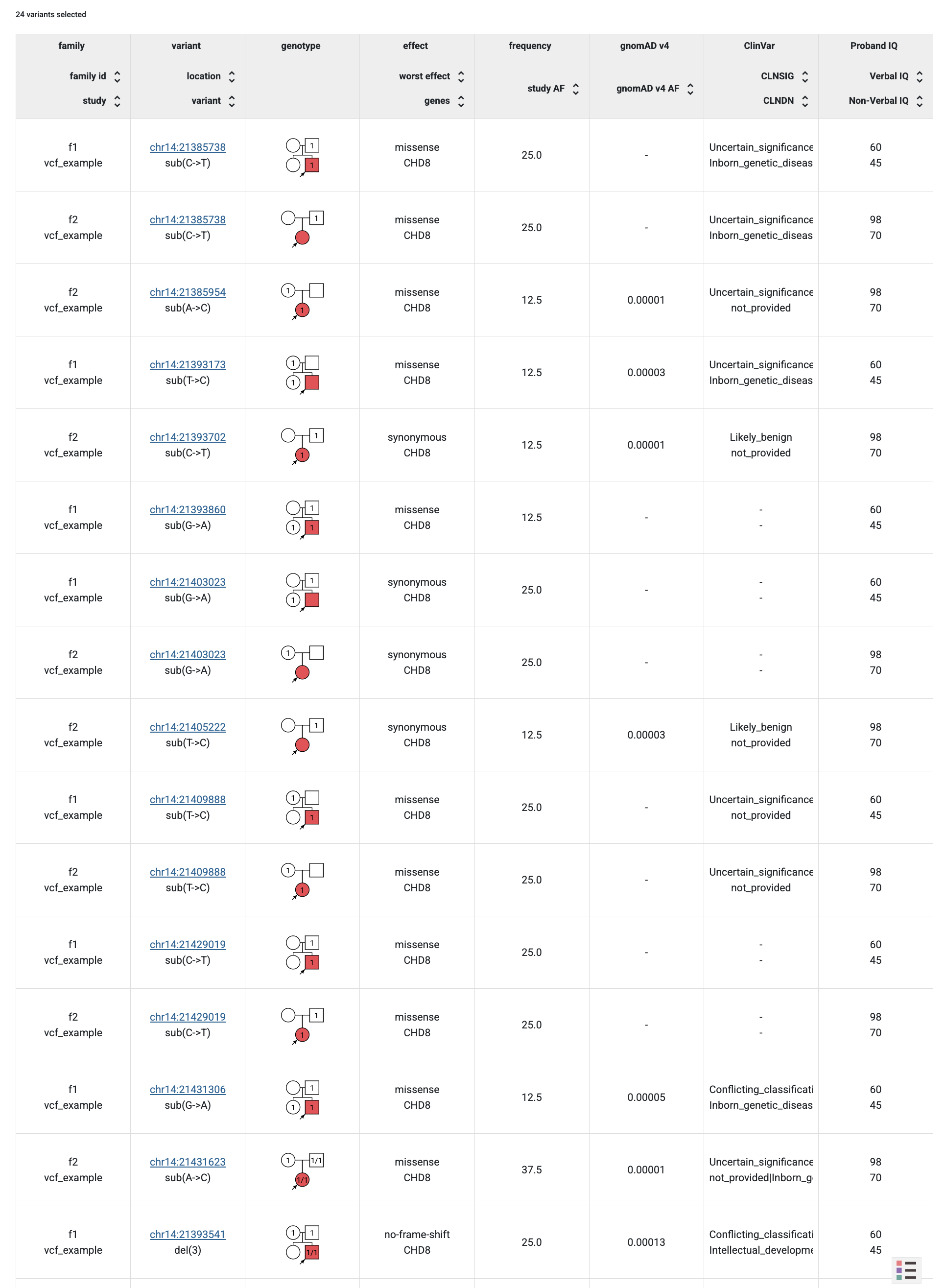
Example Dataset genotype browser using pheno measures columns
Note
For more on study configuration, see the GPF Study Configuration section.
Example import of real de Novo variants
Source of the data
As an example, let us import de novo variants from the following paper: Yoon, S., et al. Rates of contributory de novo mutation in high and low-risk autism families. Commun Biol 4, 1026 (2021).
We will focus on de novo variants from the SSC collection published in the paper mentioned above.
To import these variants into the GPF system, we need a pedigree file describing the families and a list of de novo variants.
From the supplementary data for the paper, you can download the following files:
The list of sequenced children available from Supplementary Data 1
The list of SNP and INDEL de novo variants is available from Supplementary Data 2
Note
All the data files needed for this example are available in the
gpf-getting-started
repository under the subdirectory example_imports/denovo_and_cnv_import.
Preprocess the Family Data
The list of children in Supplementary_Data_1.tsv.gz contains a lot of data
that is not relevant for the import.
We are going to use only the first five
columns from that file that look as follows:
gunzip -c Supplementary_Data_1.tsv.gz | head | cut -f 1-5 | less -S -x 20
collection          familyId            personId            affected status     sex
SSC                 11000               11000.p1            affected            M
SSC                 11000               11000.s1            unaffected          F
SSC                 11003               11003.p1            affected            M
SSC                 11003               11003.s1            unaffected          F
SSC                 11004               11004.p1            affected            M
SSC                 11004               11004.s1            unaffected          M
SSC                 11006               11006.p1            affected            M
SSC                 11006               11006.s1            unaffected          M
SSC                 11008               11008.p1            affected            M
The first column contains the collection. This study includes data from the SSC and AGRE collections. We are going to import only variants from the SSC collection.
The second column contains the family ID.
The third column contains the person’s ID.
The fourth column contains the affected status of the individual.
The fifth column contains the sex of the individual.
We need a pedigree file describing the family’s structure to import the data into GPF. The SupplementaryData1_Children.tsv.gz contains only the children; it does not include information about their parents. Fortunately for the SSC collection, it is not difficult to build the whole families’ structures from the information we have.
So, before starting the work on the import, we need to preprocess the list of children and transform it into a pedigree file.
For the SSC collection, if you have a family with ID`<fam_id>`, then the identifiers of the individuals in the family are going to be formed as follows:
mother -
<fam_id>.mo;father -
<fam_id>.fa;proband -
<fam_id>.p1;first sibling -
<fam_id>.s1;second sibling -
<fam_id>.s2.
Another essential restriction for SSC is that the only affected person in the family is the proband. The affected status of the mother, father, and siblings is unaffected.
Having this information, we can use the following Awk script to transform the list of children in a pedigree:
gunzip -c Supplementary_Data_1.tsv.gz | awk '
    BEGIN {
        OFS="\t"
        print "familyId", "personId", "dadId", "momId", "status", "sex"
    }
    $1 == "SSC" {
        fid = $2
        if( fid in families == 0) {
            families[fid] = 1
            print fid, fid".mo", "0", "0", "unaffected", "F"
            print fid, fid".fa", "0", "0", "unaffected", "M"
        }
        print fid, $3, fid".fa", fid".mo", $4, $5
    }' > ssc_denovo.ped
If we run this script, it will read Supplementary_Data_1.tsv.gz and produce
the appropriate pedigree file ssc_denovo.ped.
Note
The resulting pedigree file is also available in the
gpf-getting-started
repository under the subdirectory
example_imports/denovo_and_cnv_import.
Here is a fragment from the resulting pedigree file:
Preprocess the SNP and INDEL de Novo variants
The Supplementary_Data_2.tsv.gz file contains 255232 variants. For the import, we will use columns four and nine from this file:
gunzip -c Supplementary_Data_2.tsv.gz | head | cut -f 4,9 | less -S -x 20
personIds           variant in VCF format
13210.p1            chr1:184268:G:A
12782.s1            chr1:191408:G:A
12972.s1            chr1:271774:AG:A
12420.p1            chr1:484721:AG:A
12518.p1,12518.s1   chr1:691130:T:C
13882.p1            chr1:738645:C:G
14039.s1            chr1:819832:G:T
13872.p1            chr1:824001:AAAAT:A
Using the following Awk script, we can transform this file into easy to import the list of de Novo variants:
gunzip -c Supplementary_Data_2.tsv.gz | cut -f 4,9 | awk '
    BEGIN{
        OFS="\t"
        print "chrom", "pos", "ref", "alt", "person_id"
    }
    NR > 1 {
        split($2, v, ":")
        print v[1], v[2], v[3], v[4], $1
    }' > ssc_denovo.tsv
This script will produce a file named ssc_denovo.tsv with the following
content:
Note
The resulting ssc_denovo.tsv file is also available in the
gpf-getting-started
repository under the subdirectory
example_imports/denovo_and_cnv_import/input_data.
Caching GRR
Now we are about to import 255K variants. During the import, the GPF system will annotate these variants using the GRR resources from our public GRR. For small studies with few variants, this approach is quite convenient. However, for larger studies, it is better to cache the GRR resources locally.
To do this, we need to configure the GPF to use a local cache. Create a file
named .grr_definition.yaml in your home directory with the following
content:
id: "seqpipe"
type: "url"
url: "https://grr.iossifovlab.com"
cache_dir: "<path_to_your_cache_dir>"
The cache_dir parameter specifies the directory where the GRR resources
will be cached. The cache directory should be specified as an absolute path.
For example, /tmp/grr_cache or /Users/lubo/grrCache.
To download all the resources needed for our minimal_instance annotation,
run the following command from the gpf-getting-started directory:
grr_cache_repo -i minimal_instance/gpf_instance.yaml
Note
The grr_cache_repo command will download all the resources needed for
the GPF instance. This may take a while, depending on your internet
connection and the number of resources your configuration requires.
The resources will be downloaded to the directory specified in the
cache_dir parameter in the .grr_definition.yaml file.
For the gpf-getting-started repository, the resources that will be
downloaded are:
hg38/genomes/GRCh38-hg38hg38/gene_models/MANE/1.3hg38/variant_frequencies/gnomAD_4.1.0/genomes/ALLhg38/scores/ClinVar_20240730
The total size of the downloaded resources is about 15 GB.
Data Import of ssc_denovo
Now we have a pedigree file, ssc_denovo.ped, and a list of de novo
variants, ssc_denovo.tsv. To import this data we need to prepare an import
project. The import project is already available in the example imports
directory example_imports/denovo_and_cnv_import/ssc_denovo.yaml:
When importing genotype data, we often need to instruct the import tool how to
split the import process into multiple jobs. For this purpose, we can use
processing_config section of the import project. On lines 11-12 of the
ssc_denovo.yaml file, we have defined the processing_config section
that will split the import de Novo variants into jobs by chromosome. (For more
on import project configuration, see Import Tools.)
Note
The project file ssc_denovo.yaml is available in the the gpf-getting-started
repository under the subdirectory
example_imports/denovo_and_cnv_import.
To import the study, from the gpf-getting-started directory we should run:
time import_genotypes -v -j 10 example_imports/denovo_and_cnv_import/ssc_denovo.yaml
The -j 10 option instructs the import_genotypes tool to use 10 threads
and the -v option controls the verbosity of the output.
This command will take a while to run. The time it takes to run will depend on the number of variants in the input file and the number of threads used for the import.
Note
For example, on a MacBook Pro with the Apple M1 Pro chip, the import of the SSC de Novo variants took about 5 minutes:
real    5m29.950s
user    31m52.320s
sys     1m41.755s
When the import finishes, we can run the development GPF server:
wgpf run
In the Home page of the GPF instance, we should have the new study
ssc_denovo.
The home page has the imported SSC de Novo study.
If you follow the link to the study and choose the Genotype Browser tab, you will be able to query the imported variants.
Genotype browser for the SSC de novo variants.
Configure preview and download columns
While importing the SSC de novo variants, we used the annotation defined in the minimal instance configuration file. So, all imported variants are annotated with GnomAD and ClinVar genomic scores.
We can use these score values to define additional columns in the preview table and the download file similar to the Getting Started with Preview Columns.
Edit the ssc_denovo configuration file located at
minimal_instance/studies/ssc_denovo/ssc_denovo.yaml and add the following
snippet to the configuration file:
 1genotype_browser:
 2  column_groups:
 3    frequency:
 4      name: frequency
 5      columns:
 6      - allele_freq
 7      - gnomad_v4_genome_ALL_af
 8
 9    clinvar:
10      name: ClinVar
11      columns:
12      - CLNSIG
13      - CLNDN
14
15  preview_columns_ext:
16    - clinvar
Now, restart the GPF development server:
wgpf run
Go to the Genotype Browser tab of the ssc_denovo study and click
Preview Table button. The preview table should now contain the additional
columns for GnomAD and ClinVar genomic scores.
Genotype browser with additional columns for GnomAD and ClinVar genomic scores.
Example import of real CNV variants
Source of the data
As an example for the import of CNV variants, we will use data from the following paper: Yoon, S., et al. Rates of contributory de novo mutation in high and low-risk autism families. Commun Biol 4, 1026 (2021).
We already discussed the import of de Novo variants from this paper in Example import of real de Novo variants.
Now we will focus on the import of CNV variants from the same paper.
To import these variants into the GPF system, we need a pedigree file describing the families and a list of CNV variants.
From the supplementary data for the paper, you can download the following files:
The list of sequenced children available from Supplementary Data 1.
The list of CNV de novo variants is available from Supplementary Data 1.
Note
All the data files needed for this example are available in the
gpf-getting-started
repository under the subdirectory example_imports/denovo_and_cnv_import.
We already discussed how to transform the list of children into a pedigree file in the Preprocess the Family Data section.
Now we need to prepare the CNV variants file.
Preprocess the CNV variants
The Supplementary_Data_4.tsv.gz file contains 376 CNV variants from SSC and AGRE collections.
For the import, we will use the columns two, five, six, and seven:
gunzip -c Supplementary_Data_4.tsv.gz | cut -f 2,5-7 | less -S -x 25
collection               personIds                location                 variant
SSC                      12613.p1                 chr1:1305145-1314126     duplication
AGRE                     AU2725301                chr1:3069177-4783791     duplication
SSC                      13424.s1                 chr1:3975501-3977800     deletion
SSC                      12852.p1                 chr1:6647401-6650500     deletion
SSC                      13776.p1                 chr1:8652301-8657600     deletion
SSC                      13373.s1                 chr1:9992001-9994100     deletion
SSC                      14198.p1                 chr1:12224601-12227300   deletion
SSC                      13259.p1                 chr1:15687701-15696200   deletion
SSC                      14696.s1                 chr1:30388501-30398807   deletion
Using the following Awk script, we will filter only variants from SSC collection:
gunzip -c Supplementary_Data_4.tsv.gz | cut -f 2,5-7 | awk '
    BEGIN{
        OFS="\t"
        print "location", "variant", "person_id"
    }
    $1 == "SSC" {
        print $3, $4, $2
    }' > ssc_cnv.tsv
This script will produce a file named ssc_cnv.tsv with the following
content:
Note
The resulting ssc_cnv.tsv file is available in the
gpf-getting-started
repository under the subdirectory
example_imports/denovo_and_cnv_import/input_data.
Data Import of ssc_cnv
Now we have a pedigree file, ssc_denovo.ped, and a list of CNV
variants, ssc_cnv.tsv. To import the data we need an import project. The
import project for import ssc_cnv data is already available in the
examples directory example_imports/denovo_and_cnv_import/ssc_cnv.yaml:
Lines 12-14 configure how the CNV variants are defined in the input file.
The variant
specifies the type of the variant and values deletion and duplication
are used to define the CNV variant type.
Note
The project file ssc_cnv.yaml is available in the the gpf-getting-started
repository under the subdirectory
example_imports/denovo_and_cnv_import.
To import the study, from the gpf-getting-started directory we should run:
time import_genotypes -v -j 1 example_imports/denovo_and_cnv_import/ssc_cnv.yaml
When the import finishes, we can run the development GPF server:
wgpf run
In the Home page of the GPF instance, we should have the new
study ssc_cnv.
Home page with the imported ssc_cnv study.
If you follow the link to the ssc_cnv study and choose
the Genotype Browser tab, you
will be able to query the imported CNV variants.
Genotype browser for the SSC CNV variants.
Example import of real phenotype data
Source of the data
As an example, let us import phenotype data from the following paper: Iossifov, I., O’Roak, B., Sanders, S. et al. The contribution of de novo coding mutations to autism spectrum disorder. Nature 515, 216-221 (2014).
We will focus on the phenotype data available from the paper.
To import the phenotype data into the GPF system, we need a pedigree file describing the families and instrument files with phenotype measures.
Information about the families and the phenotype measures is available in the Supplementary Table 1 of the paper.
All supplementary data files are available from the Nature website
Note
All the data needed for this example are available in the
gpf-getting-started
repository under the subdirectory example_imports/pheno_import.
Preprocess the Family Data
The list of children in Supplementary_Table_1.tsv.gz contains both
descriptions of families, phenotype measures, and some other information,
that we do not need for the import.
We will construct the pedigree file from the first four columns of the
Supplementary_Table_1.tsv.gz file.
gunzip -c example_imports/pheno_import/Supplementary_Table_1.tsv.gz | \
    head | cut -f 1-4 | less -S -x 20
familyId            collection          probandGender       siblingGender
11542               ssc                 F                   F
13736               ssc                 M                   M
13735               ssc                 M                   F
13734               sac                 F                   M
11546               ssc                 M                   M
11547               ssc                 M
13731               ssc                 M
11545               ssc                 M
11549               ssc                 M                   F
The procedure will be similar to one already described in Preprocess the Family Data and will rely on the the specific structure of the families in the SSC collection described there.
An example Awk script to transform the Supplementary Table 1 into a pedigree file is given below.
gunzip -c example_imports/pheno_import/Supplementary_Table_1.tsv.gz | cut -f 1-4 | awk '
    BEGIN {
        OFS="\t"
        print "familyId", "personId", "dadId", "momId", "status", "sex"
    }
    $2 == "ssc" {
        fid = $1
        if( fid in families == 0) {
            families[fid] = 1
            print fid, fid".mo", "0", "0", "unaffected", "F"
            print fid, fid".fa", "0", "0", "unaffected", "M"
            print fid, fid".p1", fid".fa", fid".mo", "affected", $3
            if ($4 != "") {
                print fid, fid".s2", fid".fa", fid".mo", "unaffected", $4
            }
        }
    }' > example_imports/pheno_import/ssc_pheno.ped
If we run this script, it will read Supplementary_Table_1.tsv.gz and
produce the appropriate pedigree file ssc_pheno.ped.
Note
The resulting pedigree file is also available in the
gpf-getting-started
repository under the subdirectory
example_imports/pheno_import.
Here is a fragment from the resulting pedigree file:
Preprocess the available phenotype measures
The Supplementary_Table_1.tsv.gz file contains some phenotype measures that we will use for the import. We will focus on columns 1 and 8-13 of the file.
gunzip -c example_imports/pheno_import/Supplementary_Table_1.tsv.gz | \
    head | cut -f 1,8-13 | less -S -x 35
familyId                           motherRace                         fatherRace                         probandVIQ                         probandNVIQ                        motherAgeInMonthsAtBirthOfProband  fatherAgeInMonthsAtBirthOfProband
11542                              more-than-one-race                 white                              121                                102                                429                                430
13736                              white                              white                              119                                112                                396                                400
13735                              asian                              asian                              30                                 27                                 386                                463
13734                              white                              white                              36                                 51                                 368                                348
11546                              white                              white                              100                                123                                437                                406
11547                              asian                              asian                              49                                 49                                 380                                434
13731                              white                              white                              115                                113                                367                                491
11545                              white                              white                              83                                 114                                383                                441
11549                              african-amer                       african-amer                       36                                 61                                 406                                481
The available measures are as follows:
motherRace: mother’s race.fatherRace: father’s race.probandVIQ: proband’s verbal IQ.probandNVIQ: proband’s non-verbal IQ.motherAgeInMonthsAtBirthOfProband: mother’s age in months at the birth of the proband.fatherAgeInMonthsAtBirthOfProband: father’s age in months at the birth of the proband.
Using the following Awk script, we will extract the relevant measures into an instrument file.
gunzip -c example_imports/pheno_import/Supplementary_Table_1.tsv.gz | cut -f 1,8-13 | awk '
    BEGIN {
        OFS=","
        print "individual", "motherRace", "fatherRace", "probandVIQ", "probandNVIQ", "motherAgeInMonthsAtBirthOfProband", "fatherAgeInMonthsAtBirthOfProband"
    }
    $1 != "familyId" {
        print $1".p1", $2, $3, $4, $5, $6, $7, $8
    }' > example_imports/pheno_import/proband_measures.csv
This script will produce a file named proband_measures.csv with the
following content:
individual |
motherRace |
fatherRace |
probandVIQ |
probandNVIQ |
motherAgeInMonthsAtBirthOfProband |
fatherAgeInMonthsAtBirthOfProband |
|
|---|---|---|---|---|---|---|---|
11542.p1 |
more-than-one-race |
white |
121 |
102 |
429 |
430 |
|
13736.p1 |
white |
white |
119 |
112 |
396 |
400 |
|
13735.p1 |
asian |
asian |
30 |
27 |
386 |
463 |
|
13734.p1 |
white |
white |
36 |
51 |
368 |
348 |
|
11546.p1 |
white |
white |
100 |
123 |
437 |
406 |
|
11547.p1 |
asian |
asian |
49 |
49 |
380 |
434 |
|
13731.p1 |
white |
white |
115 |
113 |
367 |
491 |
|
11545.p1 |
white |
white |
83 |
114 |
383 |
441 |
|
11549.p1 |
african-amer |
african-amer |
36 |
61 |
406 |
481 |
|
13739.p1 |
white |
white |
16 |
35 |
464 |
467 |
Note
The resulting file proband_measures.csv is also available in the
gpf-getting-started
repository under the subdirectory
example_imports/pheno_import.
Data Import of ssc_pheno
Now we have a pedigree file, ssc_pheno.ped, and an instrument file
proband_measures.csv. To import this data, we need an import
project. A suitable import project is already available in the example imports
directory example_imports/pheno_import/ssc_pheno.yaml:
To import the phenotype data, we will use the import_phenotypes tool.
import_phenotypes example_imports/pheno_import/ssc_pheno.yaml
When the import finishes, we can run the GPF development server using:
wgpf run
Now, on the GPF instance Home Page, you should see the ssc_pheno
phenotype study. If you follow the link, you will see the Phenotype Browser
tab with the imported data.
Phenotype Browser with imported phenotype study ssc_pheno
Configure a genotype study ssc_denovo to use phenotype data
Now we can configure the ssc_denovo genotype study to use the newly
import phenotype data. We need to edit the ssc_denovo.yaml configuration
file located in the minimal_instance/studies/ssc_denovo/ directory and
add line 18 as shown below:
 1id: ssc_denovo
 2conf_dir: .
 3has_denovo: true
 4has_cnv: false
 5has_transmitted: false
 6genotype_storage:
 7  id: internal
 8  tables:
 9    pedigree: parquet_scan('ssc_denovo/pedigree/pedigree.parquet')
10    meta: parquet_scan('ssc_denovo/meta/meta.parquet')
11    summary: parquet_scan('ssc_denovo/summary/*.parquet')
12    family: parquet_scan('ssc_denovo/family/*.parquet')
13genotype_browser:
14  enabled: true
15denovo_gene_sets:
16  enabled: true
17
18phenotype_data: ssc_pheno
When you restart the GPF instance, you should be able to see
Phenotype Browser and the Phenotype Tool tabs enabled for the
ssc_denovo study.
Genotype study ssc_denovo with phenotype data configured.
Now we can use the Phenotype Tool to see how de Novo variants are correlated with the proband’s phenotype measures.
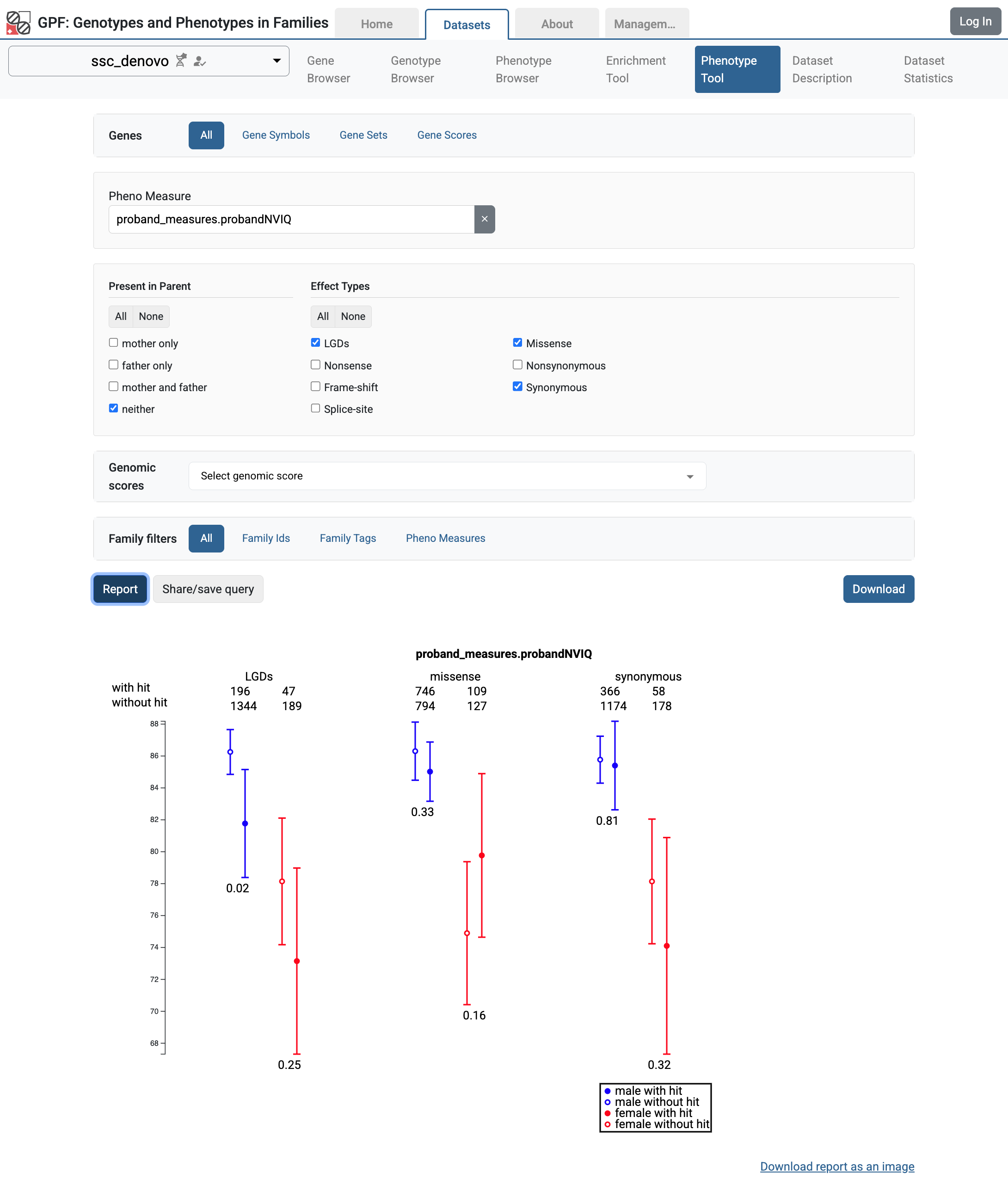
Phenotype Tool results for the proband non-verbal IQ in ssc_denovo study.
Getting Started with Gene Sets and Gene Scores
The GPF system provides support for the collection of gene symbols of interest for the analysis of genotype data. There are two types of gene sets that can be used in GPF:
de Novo gene sets - for each genotype study that has de Novo variants, the GPF system can create gene sets that contain a list of genes with de Novo variants of interest; for example, genes with LGSs de Novo variants, genes with LGDs de Novo variants in males, etc.
pre-defined gene sets - these are gene sets that are defined in the GRR used by the GPF instance; for example, in the public GPF Genomic Resources Repository (GRR) there are multiple gene set collections ready for use in the GPF instance.
De Novo Gene Set
By default, for each genotype study with de Novo variants, the GPF system creates a collection of de Novo gene sets with pre-defined properties. For example:
LGDs - genes with LGDs de Novo variants;
LGDs.Female - genes with LGDs de Novo variants in females;
LGDs.Male - genes with LGDs de Novo variants in males;
Missense - genes with missense de Novo variants;
Missense.Female - genes with missense de Novo variants in females;
Missense.Male - genes with missense de Novo variants in males;
etc.
You can use these gene sets in multiple tools in the GPF system. For example,
if you navigate to Genotype Browser for ssc_denovo study,
and select the Genes > Gene Sets tab, you will see the list of de Novo gene
sets generated for the study.
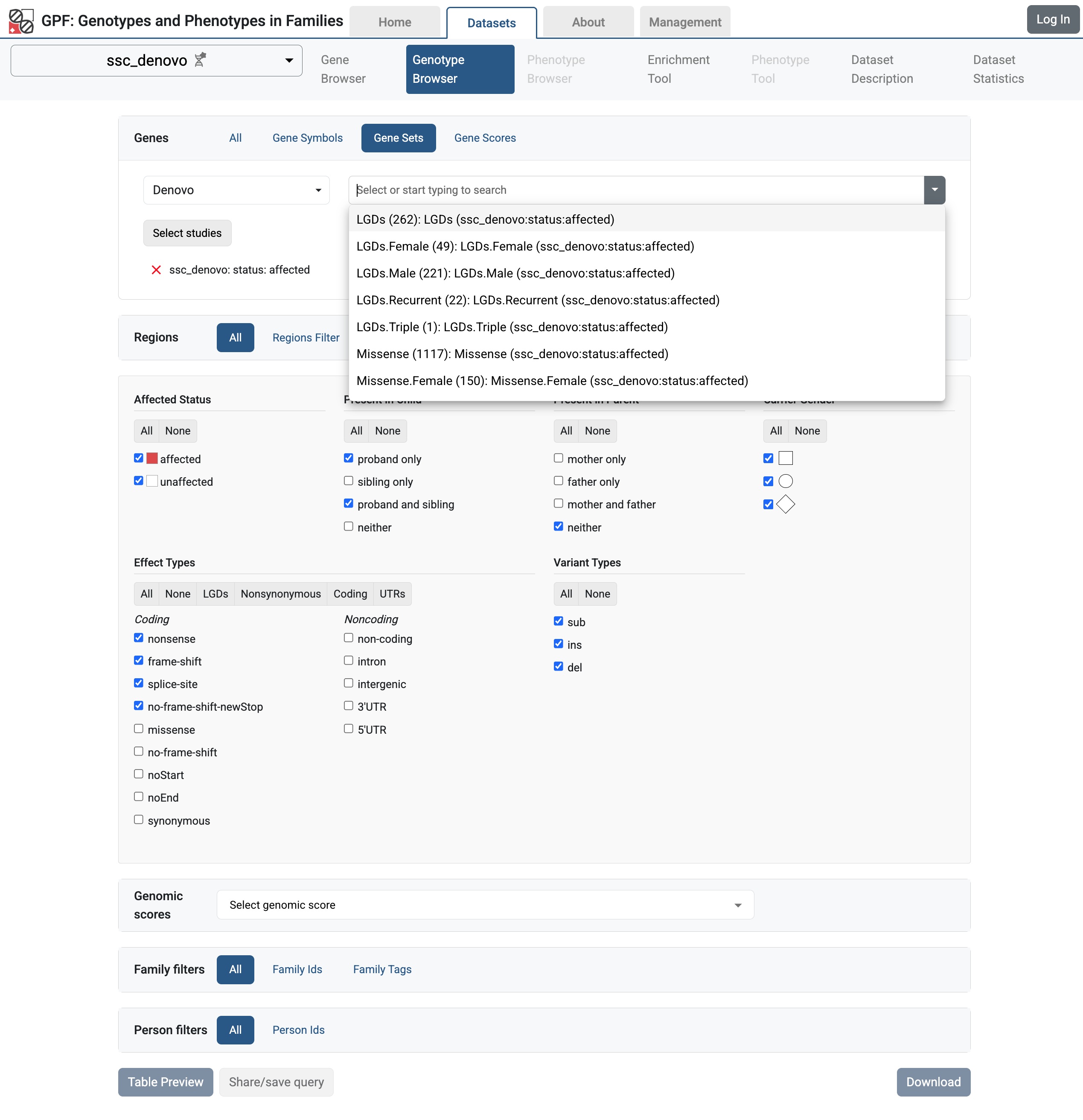
De Novo Gene Sets for ssc_denovo study
You can use these gene sets in the Genotype Browser to filter the variants in genes that are included in the selected gene set.
Pre-defined Gene Set Collections
To add pre-defined gene sets from the GRR to the GPF instance, you need to edit
the GPF instance configuration file (minimal_instance/gpf_instance.yaml).
Let’s say that we want to add the following gene set collections from the public GRR:
gene_properties/gene_sets/autism - autism gene sets derived from publications;
gene_properties/gene_sets/relevant - variety of gene sets with potential relevance to autism;
gene_properties/gene_sets/GO_2024-06-17_release - this gene set collection contains genes associated with Gene Ontology (GO) terms.
To do this, you need to add lines 14-18 to the GPF instance configuration file
(minimal_instance/gpf_instance.yaml):
 1instance_id: minimal_instance
 2
 3reference_genome:
 4  resource_id: "hg38/genomes/GRCh38-hg38"
 5
 6gene_models:
 7  resource_id: "hg38/gene_models/MANE/1.3"
 8
 9annotation:
10  config:
11    - allele_score: hg38/variant_frequencies/gnomAD_4.1.0/genomes/ALL
12    - allele_score: hg38/scores/ClinVar_20240730
13
14gene_sets_db:
15  gene_set_collections:
16  - gene_properties/gene_sets/autism
17  - gene_properties/gene_sets/relevant
18  - gene_properties/gene_sets/GO_2024-06-17_release
When you restart the GPF instance, the configured gene set collections will be
available in the GPF instance user interface. For example, if you navigate to
Genotype Browser for ssc_denovo study,
and select the Genes > Gene Sets tab, you will see the configured gene set
collections.
Gene Set Collections in the ssc_denovo Genotype Browser interface
Pre-defined Gene Scores
To add pre-defined gene scores from the GRR to the GPF instance, you need to
edit the GPF instance configuration file
(minimal_instance/gpf_instance.yaml).
Let’s say that we want to add the following gene set collections from the public GRR:
gene_properties/gene_scores/Satterstrom_Buxbaum_Cell_2020 TADA derived gene-autism association score
gene_properties/gene_scores/Iossifov_Wigler_PNAS_2015 Probability of a gene to be associated with autism
gene_properties/gene_scores/LGD Gene vulnerability/intolerance score based on the rare LGD variants
gene_properties/gene_scores/RVIS Residual Variation Intolerance Score
gene_properties/gene_scores/LOEUF Degree of intolerance to predicted Loss-of-Function (pLoF) variation
To do this, you need to add lines 20-26 to the GPF instance configuration file
(minimal_instance/gpf_instance.yaml):
 1instance_id: minimal_instance
 2
 3reference_genome:
 4  resource_id: "hg38/genomes/GRCh38-hg38"
 5
 6gene_models:
 7  resource_id: "hg38/gene_models/MANE/1.3"
 8
 9annotation:
10  config:
11    - allele_score: hg38/variant_frequencies/gnomAD_4.1.0/genomes/ALL
12    - allele_score: hg38/scores/ClinVar_20240730
13
14gene_sets_db:
15  gene_set_collections:
16  - gene_properties/gene_sets/autism
17  - gene_properties/gene_sets/relevant
18  - gene_properties/gene_sets/GO_2024-06-17_release
19
20gene_scores_db:
21  gene_scores:
22  - gene_properties/gene_scores/Satterstrom_Buxbaum_Cell_2020
23  - gene_properties/gene_scores/Iossifov_Wigler_PNAS_2015
24  - gene_properties/gene_scores/LGD
25  - gene_properties/gene_scores/RVIS
26  - gene_properties/gene_scores/LOEUF
When you restart the GPF instance, the configured gene scores will be
available in the GPF instance user interface. For example, if you navigate to
Genotype Browser for ssc_denovo study,
and select the Genes > Gene Scores tab, you will see the configured gene set
collections.
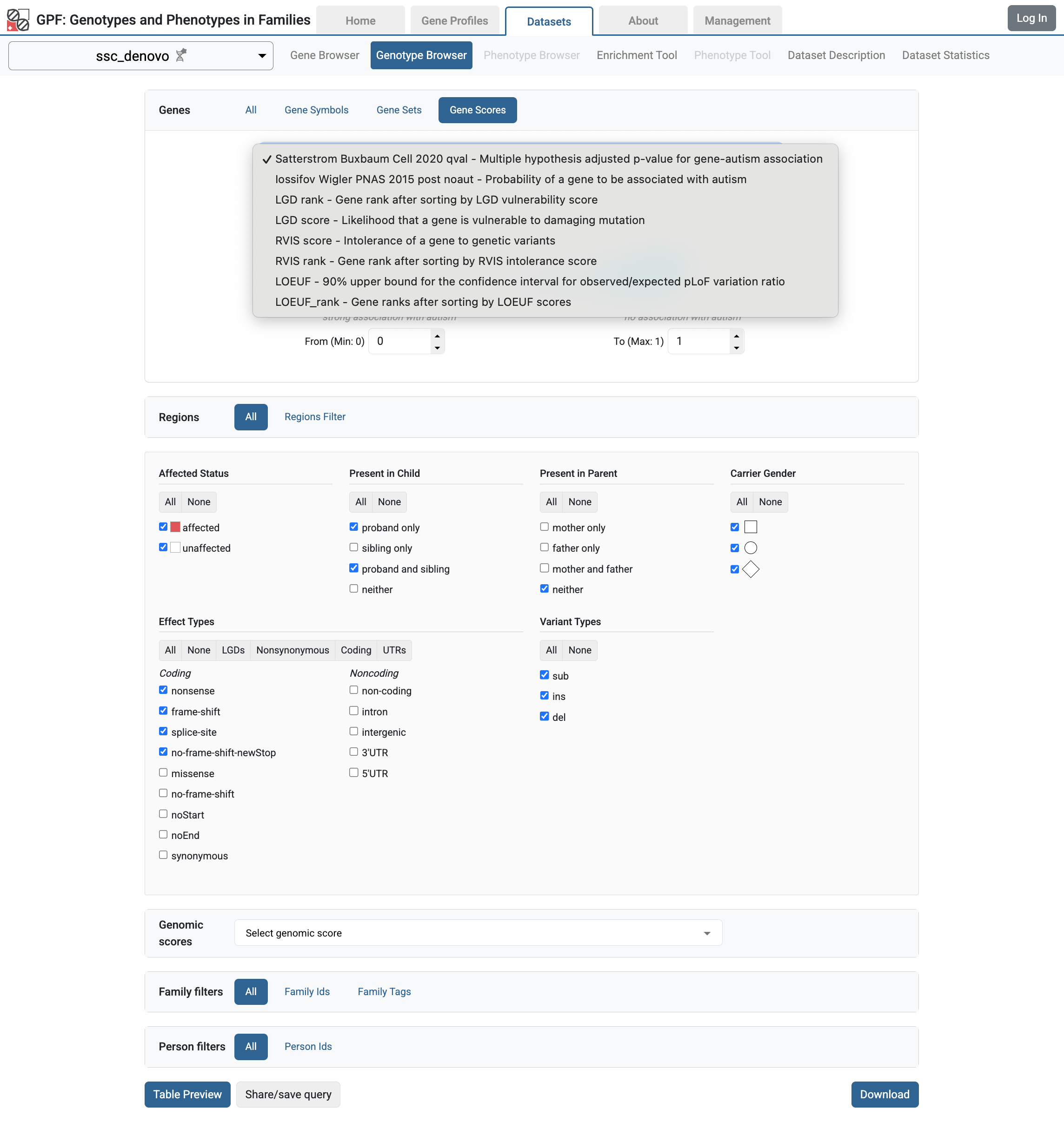
Gene Scores in the ssc_denovo Genotype Browser interface
Getting Started with Enrichment Tool
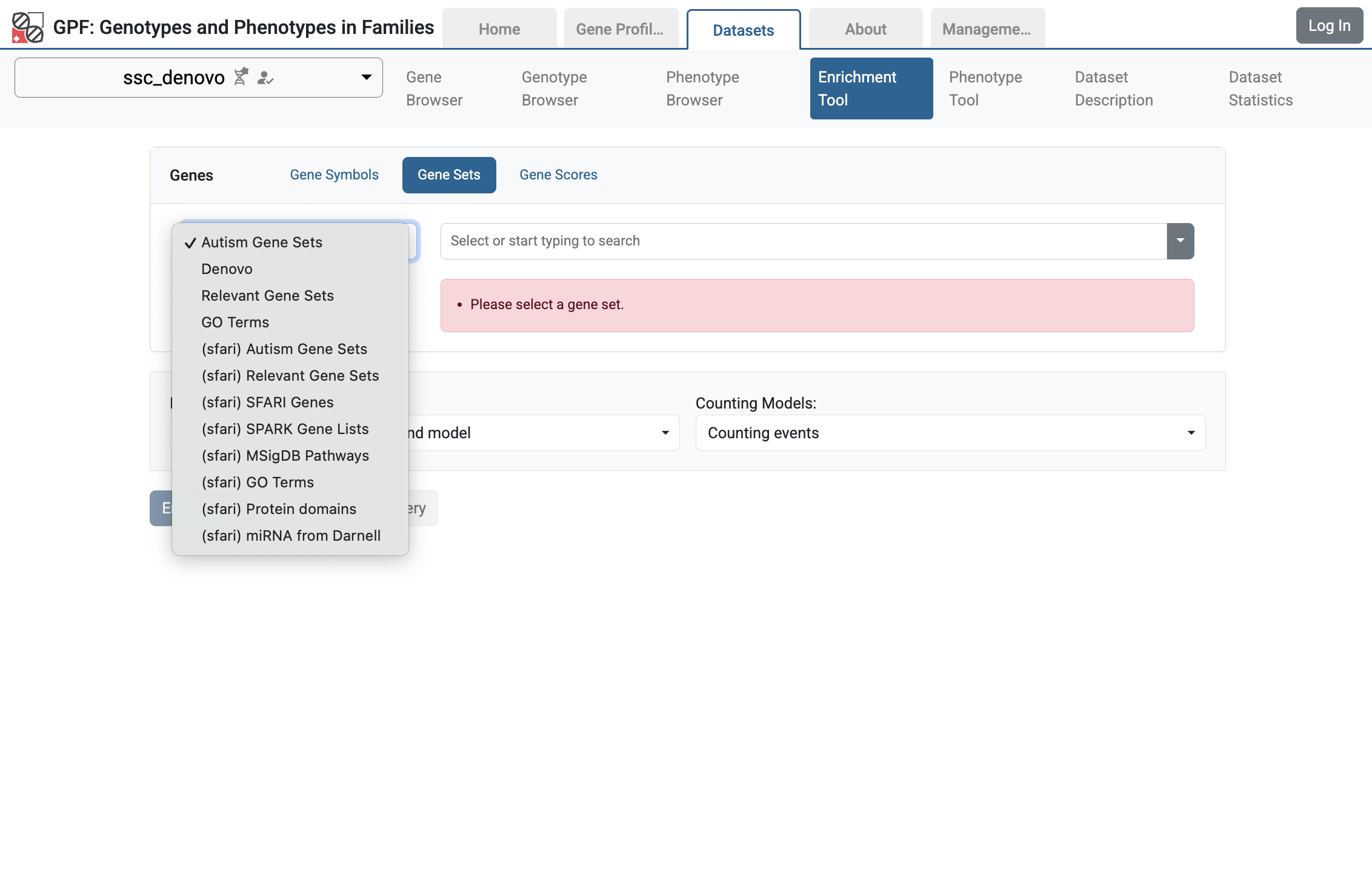
By default, for each genotype study with de Novo variants, the GPF system enables the Enrichment tool.
The Enrichment Tool allows the user to test if a given set of genes is affected by more or fewer de novo mutations in the children than expected.
To use the Enrichment Tool, a user must choose a set of genes either by selecting one of the gene sets that have already been configured in GPF or by providing their own list of gene symbols.
The user also must select among the background models that GPF uses to compute the expected number of de novo mutations within the given dataset.
Note
By default, for studies with de Novo variants, only one background model is configured: enrichment/samocha_background
To use other background models, the user must edit the study configuration file.
If you navigate to the Enrichment Tool page for the ssc_denovo study,
you will be able to use the tool with run different tests.
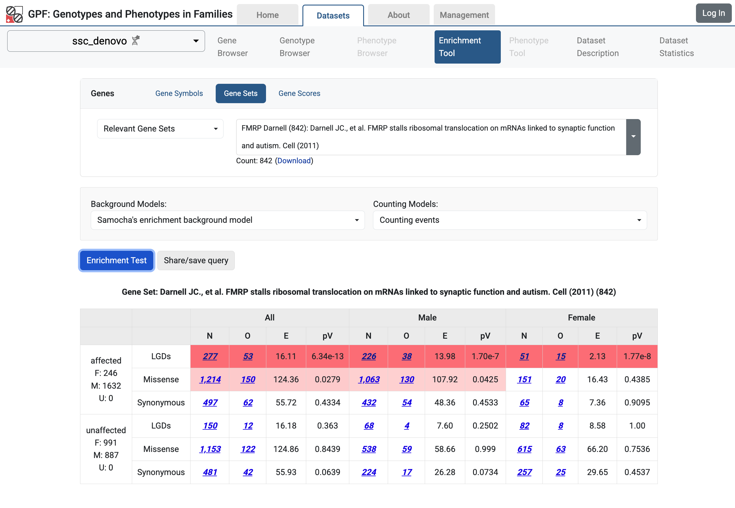
Enrichment Tool for ssc_denovo study.
Getting Started with Gene Profiles
The Gene Profile tool provides summary statistics of the data managed by GPF and additional relevant information organized by gene.
To enable the Gene Profile tool, you need to create a configuration for the tool and add it to the GPF instance configuration file.
Let us create a configuration for the Gene Profile tool in the GPF instance
directory minimal_instance/gene_profiles.yaml with the following content:
 1datasets:
 2  ssc_denovo:
 3    statistics:
 4    - id: denovo_lgds
 5      description: de Novo LGDs
 6      display_name: dn LGDs
 7      effects:
 8      - LGDs
 9      category: denovo
10    - id: denovo_missense
11      description: de Novo missense
12      display_name: dn mis
13      effects:
14      - missense
15      category: denovo
16      default_visible: true
17    - id: denovo_intronic_indels
18      description: number of de Novo intronic indels
19      display_name: dn IIND
20      effects:
21      - intron
22      category: denovo
23      variant_types:
24      - ins
25      - del
26      default_visible: true
27    person_sets:
28    - set_name: affected
29      collection_name: status
30      default_visible: true
31    - set_name: unaffected
32      collection_name: status
33      default_visible: true
34
35gene_scores:
36- category: autism_scores
37  display_name: Autism Gene Scores
38  scores:
39  - score_name: Satterstrom Buxbaum Cell 2020 qval
40    format: "%%.2f"
41  - score_name: Iossifov Wigler PNAS 2015 post noaut
42    format: "%%.2f"
43
44- category: protection_scores
45  display_name: Protection Gene Scores
46  scores:
47    - score_name: RVIS_rank
48      format: "%%s"
49    - score_name: LGD_rank
50      format: "%%s"
51    - score_name: LOEUF_rank
52      format: "%%s"
53
54gene_sets:
55- category: autism_gene_sets
56  display_name: Autism Gene Sets
57  sets:
58  - set_id: autism candidates from Iossifov PNAS 2015
59    collection_id: autism
60  - set_id: autism candidates from Sanders Neuron 2015
61    collection_id: autism
62  - set_id: Yuen Scherer Nature 2017
63    collection_id: autism
64  - set_id: Turner Eichler ajhg 2019
65    collection_id: autism
66  - set_id: Satterstrom Buxbaum Cell 2020 top
67    collection_id: autism
68
69gene_links:
70- name: Gene Browser
71  url: "datasets/ssc_denovo/gene-browser/{gene}"
72
73- name: GeneCards
74  url: "https://www.genecards.org/cgi-bin/carddisp.pl?gene={gene}"
75- name: SFARI gene
76  url: "https://gene.sfari.org/database/human-gene/{gene}"
77
78default_dataset: ssc_denovo
79
80order:
81- autism_gene_sets_rank
82- autism_scores
83- ssc_denovo
84- protection_scores
There are several sections in this configuration file:
datasets: This section defines the studies and datasets that will be used to collect variant statistics. In our example, we are going to use thessc_denovostudy - see lines 2-33.For each study or dataset, we should define what type of variant statistics we want to collect. In our example, we are going to collect three types of statistics:
Count of LGDs de Novo variants for each gene - lines 4-9;
Count of missense de Novo variants for each gene - lines 10-16;
Count of intronic INDEL variants for each gene - lines 17-26.
For each study or dataset, we should define how to split individuals into groups. In our example, we are going to split them into two groups -
affectedandunaffected- lines 27-33.
gene_scores: This section defines groups of gene scores that will be used in gene profiles. The gene profiles will include score values for each gene from the defined gene scores. In our example, we are going to use two groups of gene scores:autism_scores- lines 36-42;protection_scores- lines 44-52.
Please note that all gene scores used in this configuration section should be defined in the GPF instance configuration file.
gene_sets: This section defines groups of gene sets that will be used in gene profiles. The gene profiles will show if the gene is included in the defined gene sets. In our example, we are going to use one group of gene sets:autism_gene_sets- lines 54-67;Please note that all gene sets used in this configuration section should be defined in the GPF instance configuration file.
gene_links: This section defines links to internal and external tools that contain information about genes. In our example, we are defining three links: - lines 70-71 - link to the GPF Gene Browser tools; - lines 73-74 - link to the GeneCards site; - lines 75-76 - link to the SFARI Gene site.
Once we have this configuration, we need to add it to the GPF instance configuration:
 1instance_id: minimal_instance
 2
 3reference_genome:
 4  resource_id: "hg38/genomes/GRCh38-hg38"
 5
 6gene_models:
 7  resource_id: "hg38/gene_models/MANE/1.3"
 8
 9annotation:
10  config:
11    - allele_score: hg38/variant_frequencies/gnomAD_4.1.0/genomes/ALL
12    - allele_score: hg38/scores/ClinVar_20240730
13
14gene_sets_db:
15  gene_set_collections:
16  - gene_properties/gene_sets/autism
17  - gene_properties/gene_sets/relevant
18  - gene_properties/gene_sets/GO_2024-06-17_release
19
20gene_scores_db:
21  gene_scores:
22  - gene_properties/gene_scores/Satterstrom_Buxbaum_Cell_2020
23  - gene_properties/gene_scores/Iossifov_Wigler_PNAS_2015
24  - gene_properties/gene_scores/LGD
25  - gene_properties/gene_scores/RVIS
26  - gene_properties/gene_scores/LOEUF
27
28gene_profiles_config:
29  conf_file: gene_profiles.yaml
Once we have configured the GPF Gene Profiles, we need to prebuild the
gene profiles. The prebuilding of the gene profiles is done using the
generate_gene_profile command. By default, the generate_gene_profiles
command will generate profiles for all genes in the GPF instance gene models.
The gene models we are using in our example hg38/gene_models/MANE/1.3
have 19,285 genes. Please note that generating gene profiles for all genes
will take a while to finish. On a MacBook Pro M1 with 32GB of RAM,
it took about 10 minutes to finish.
generate_gene_profile
Note
If you want to speed up the process of generating gene profiles, you can limit the number of genes for which the profiles will be generated. For example, in the following command, we are generating gene profiles for a list of ten genes:
generate_gene_profile \
    --genes \
    CHD8,NCKAP1,DSCAM,ANK2,GRIN2B,SYNGAP1,ARID1B,MED13L,GIGYF1,WDFY3
Once the generation of gene profiles is finished, you can start the GPF
instance using the wgpf command:
wgpf run
On the home page of the GPF instance, you should be able to see Gene Profiles tool:
Gene Profiles tool links added to the GPF instance home page
If you follow the All Genes link from the Home Page, you will be taken to the Gene Profiles table with information about genes.
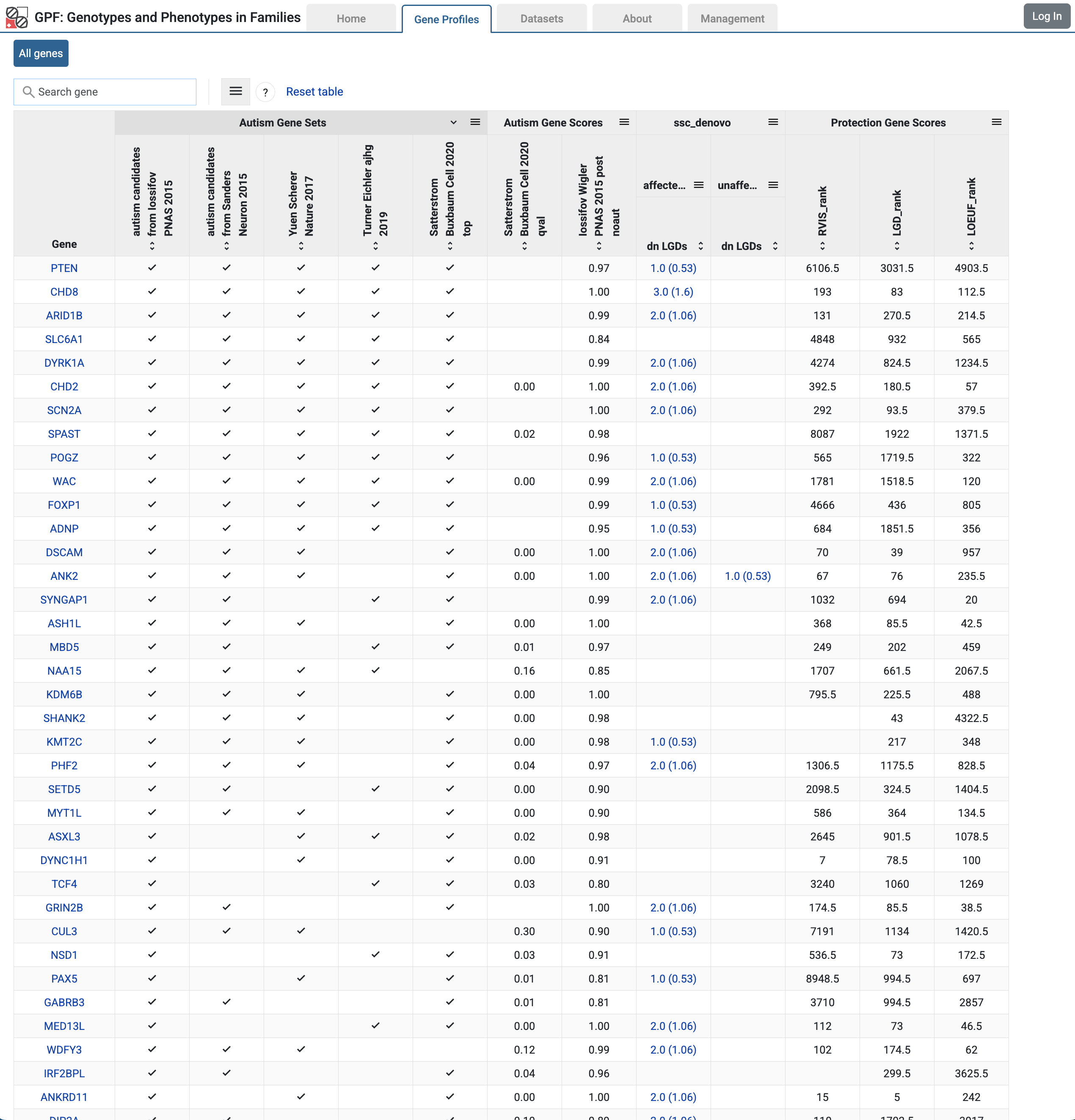
Gene Profiles table with summary information about genes
If you select a gene from the table, the GPF will open the Gene Profile page for the selected gene.
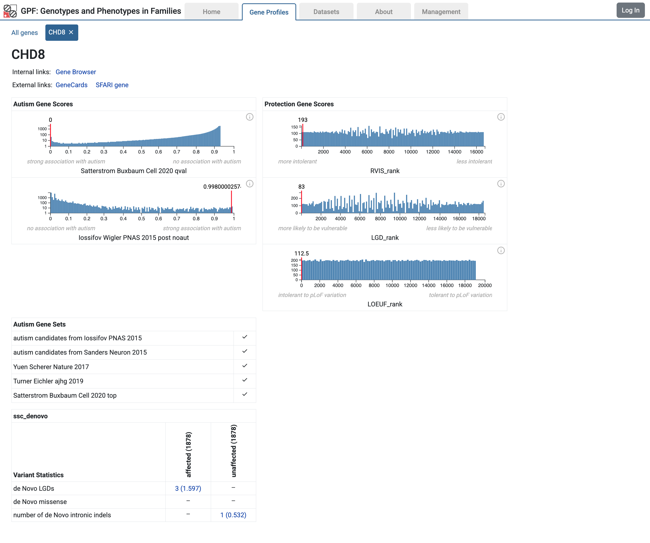
Gene Profile page for the CHD8 gene
Note
For more information about the Gene Profile tool, please refer to the user interface documentation Gene Profiles.
Getting Started with Federation
Federation is a mechanism that allows you to combine multiple GPF instances into a single system. This allows you to share data and resources across multiple GPF instances, enabling you to work with larger datasets and collaborate with other researchers more effectively.
In this section, we will show you how to set up a federation between the SFARI GPF instance and your local GPF instance. This will allow you to access the data and resources you have access to on the SFARI GPF instance from your local GPF instance.
Configure federation on your local GPF instance
To use the GPF federation, you need to install the additional
gpf_federation conda package in your local conda environment. You can do
this by running the following command:
mamba install \
    -c conda-forge \
    -c bioconda \
    -c iossifovlab \
    gpf_federation
Once the package is installed, you need to configure the federation on your
local GPF instance. You can do this by editing the
minimal_instacne/gpf_instance.yaml file:
 1instance_id: minimal_instance
 2
 3reference_genome:
 4  resource_id: "hg38/genomes/GRCh38-hg38"
 5
 6gene_models:
 7  resource_id: "hg38/gene_models/MANE/1.3"
 8
 9annotation:
10  config:
11    - allele_score: hg38/variant_frequencies/gnomAD_4.1.0/genomes/ALL
12    - allele_score: hg38/scores/ClinVar_20240730
13
14gene_sets_db:
15  gene_set_collections:
16  - gene_properties/gene_sets/autism
17  - gene_properties/gene_sets/relevant
18  - gene_properties/gene_sets/GO_2024-06-17_release
19
20gene_scores_db:
21  gene_scores:
22  - gene_properties/gene_scores/Satterstrom_Buxbaum_Cell_2020
23  - gene_properties/gene_scores/Iossifov_Wigler_PNAS_2015
24  - gene_properties/gene_scores/LGD
25  - gene_properties/gene_scores/RVIS
26  - gene_properties/gene_scores/LOEUF
27
28gene_profiles_config:
29  conf_file: gene_profiles.yaml
30
31remotes:
32  - id: "sfari"
33    url: "https://gpf.sfari.org/hg38"
Note
This configuration will allow your local instance to access only the publicly available resources in the SFARI GPF instance.
In case you have a user account on the SFARI GPF instance, you can create federation tokens and use them to access the remote instance as described in the Federation tokens.
When you are ready with the configuration, you can start the GPF instance using
the wgpf tool:
wgpf run
On the home page of your local GPF instance, you should see studies loaded from the SFARI remote instance in the Home Page:
Home page with studies from the SFARI GPF instance
Warning
The federation loads a lot of data from the remote instance. When you start the GPF instance, it may take some time to load all the needed information.
Combine analysis using local and remote studies
Having the federation configured, you can explore local and remote studies. Moreover, you can combine local and remote studies using the available tools.
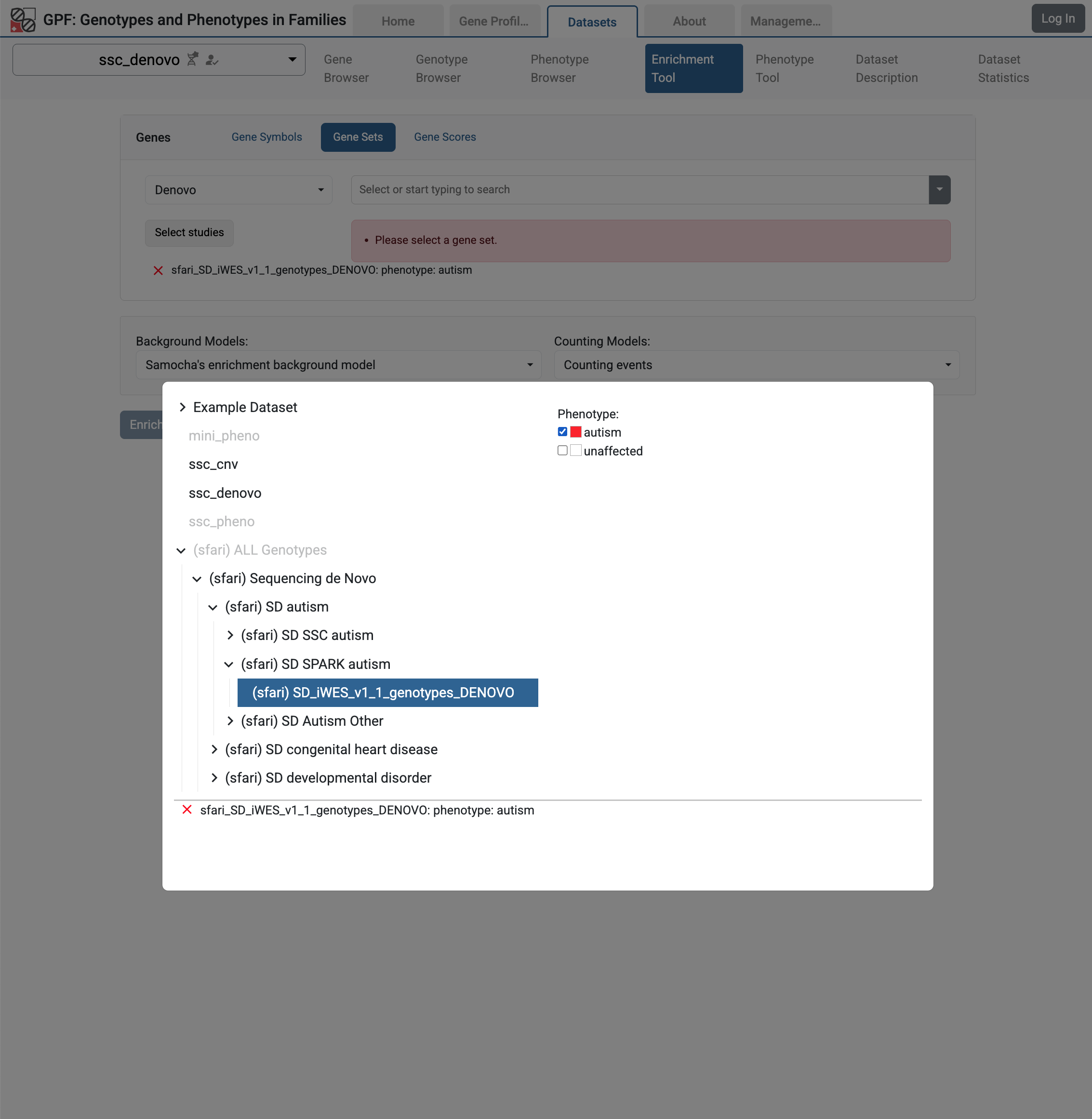
For example, let’s go to the ssc_denovo and select the Enrichment Tool. From Gene Sets choose Denovo:
Enrichment Tool for ssc_denovo study
Then from the studies hierarchy choose (sfari) Sequencing de Novo / (sfari) SD Autism / (sfari) SD SPARK Autism / (sfari) SD iWES_v1_1_genotypes_DENOVO study and select the autism phenotype.
Enrichment Tool for ssc_denovo study with selected remote study de Novo gene sets
Let us select the LGDs de Novo gene set and run the Enrichment Tool:
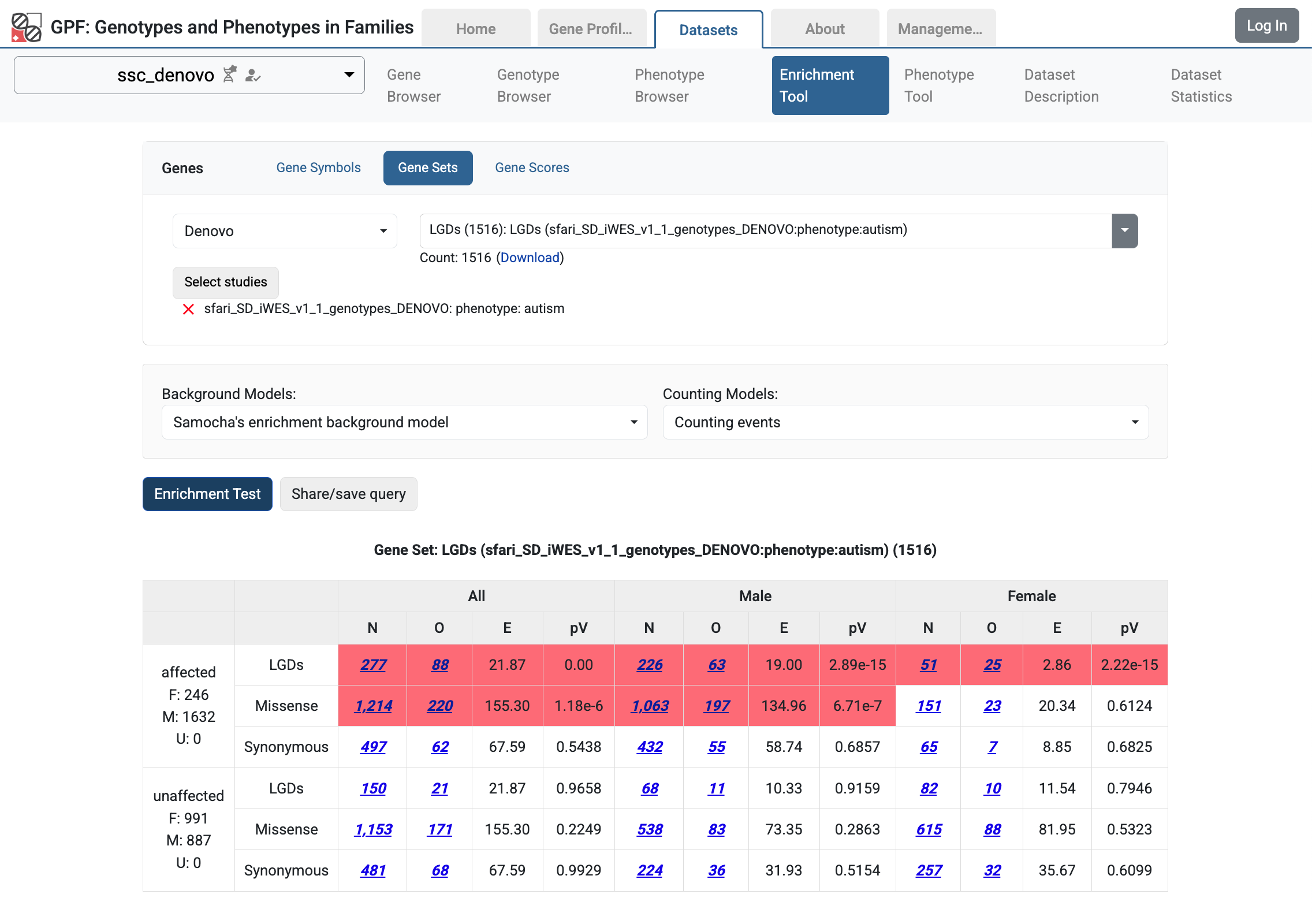
De Novo gene set from SD_iWES_v1_1_genotypes_DENOVO study
Federation tokens
Federation tokens are used to authenticate and authorize access to the federated GPF instance.
Let us create a federation token for the SFARI GPF instance. You need to log in to the SFARI GPF instance, go to User Profile, select Federation Tokens, and create a new federation token:
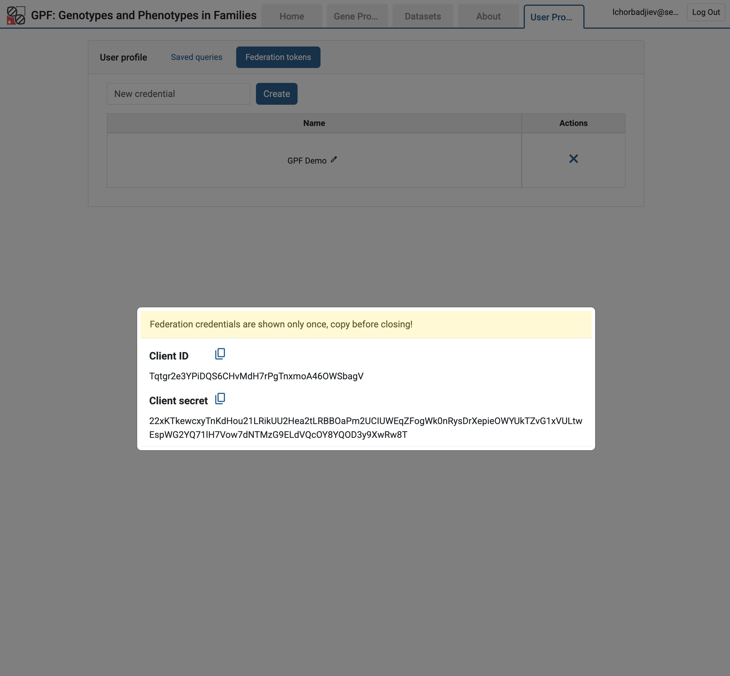
Federation client ID and secret from the User Profile
Warning
The federation client ID and secret are shown only once. Make sure to copy them to a safe place. You will need them to configure the federation on your local GPF instance.
Once you have the federation client ID and secret, you can configure your local
GPF instance to use them. You need to edit the
minimal_instance/gpf_instance.yaml file and add the lines 5-6 to the
remotes section:
1remotes:
2  - id: "sfari"
3    url: "https://gpf.sfari.org/hg38"
4    client_id: "Tqtgr2e3YPiDQS6CHvMdH7rPgTnxmoA46OWSbagV"
5    client_secret: "22xKTkewcxyTnKdHou21LRikUU2Hea2tLRBBOaPm2UCIUWEqZFogWk0nRysDrXepieOWYUkTZvG1xVULtwEspWG2YQ71lH7Vow7dNTMzG9ELdVQcOY8YQOD3y9XwRw8T"
This will allow your local GPF instance to have access to the resources in SFARI GPF instance that you have access to.
Warning
The federation client ID and secret in the example above are placeholders and should not be used. You need to replace them with your own federation client ID and secret.
Example Usage of GPF Python Interface
The simplest way to start using GPF’s Python API is to import the
GPFInstance class and instantiate it:
from dae.gpf_instance.gpf_instance import GPFInstance
gpf_instance = GPFInstance.build()
This gpf_instance object groups several interfaces, each dedicated
to managing different parts of the underlying data. It can be used to interact
with the system as a whole.
Querying genotype data
For example, to list all studies configured in the startup GPF instance, use:
gpf_instance.get_genotype_data_ids()
This will return a list with the IDs of all configured studies:
['ssc_denovo', 'denovo_example', 'vcf_example', 'ssc_cnv', 'example_dataset']
To get a specific study and query it, you can use:
st = gpf_instance.get_genotype_data('example_dataset')
vs = list(st.query_variants())
Note
The query_variants method returns a Python iterator.
To get the basic information about variants found by the query_variants
method, you can use:
for v in vs:
    for aa in v.alt_alleles:
        print(aa)
will produce the following output:
chr14:21391016 A->AT f2
chr14:21393484 TCTTC->T f2
chr14:21402010 G->A f1
chr14:21403019 G->A f2
chr14:21403214 T->C f1
chr14:21431459 G->C f1
chr14:21385738 C->T f1
chr14:21385738 C->T f2
chr14:21385954 A->C f2
chr14:21393173 T->C f1
chr14:21393702 C->T f2
chr14:21393860 G->A f1
chr14:21403023 G->A f1
chr14:21403023 G->A f2
chr14:21405222 T->C f2
chr14:21409888 T->C f1
chr14:21409888 T->C f2
chr14:21429019 C->T f1
chr14:21429019 C->T f2
chr14:21431306 G->A f1
chr14:21431623 A->C f2
chr14:21393540 GGAA->G f1
The query_variants interface allows you to specify what kind of variants
you are interested in. For example, if you only need “synonymous” variants, you
can use:
st = gpf_instance.get_genotype_data('example_dataset')
vs = st.query_variants(effect_types=['synonymous'])
vs = list(vs)
len(vs)
>> 4
Or, if you are interested in “synonymous” variants only in people with “prb” role, you can use:
vs = st.query_variants(effect_types=['synonymous'], roles='prb')
vs = list(vs)
len(vs)
>> 1
Querying phenotype data
To list all available phenotype data, use:
gpf_instance.get_phenotype_data_ids()
This will return a list with the IDs of all configured phenotype data:
['ssc_pheno', 'mini_pheno']
To get a specific phenotype data and query it, use:
pd = gpf_instance.get_phenotype_data("mini_pheno")
We can see what instruments and measures are available in the data:
pd.instruments
>> {'basic_medical': Instrument(basic_medical, 4), 'iq': Instrument(iq, 3)}
pd.measures
>> {'basic_medical.age': Measure(basic_medical.age, MeasureType.continuous, 1, 50),
    'basic_medical.weight': Measure(basic_medical.weight, MeasureType.continuous, 15, 250),
    'basic_medical.height': Measure(basic_medical.height, MeasureType.continuous, 30, 185),
    'basic_medical.race': Measure(basic_medical.race, MeasureType.categorical, african american, asian, white),
    'iq.diagnosis-notes': Measure(iq.diagnosis-notes, MeasureType.categorical, excels at school, originally diagnosed as Asperger, sleep abnormality, walked late),
    'iq.verbal-iq': Measure(iq.verbal-iq, MeasureType.continuous, 60, 115),
    'iq.non-verbal-iq': Measure(iq.non-verbal-iq, MeasureType.continuous, 45, 115)}
We can then get specific measure values for specific individuals:
from dae.variants.attributes import Role

list(pd.get_people_measure_values(["iq.non-verbal-iq"], roles=[Role.prb], family_ids=["f1", "f2", "f3"]))
>> [{'person_id': 'f1.p1',
     'family_id': 'f1',
     'role': 'prb',
     'status': 'affected',
     'sex': 'M',
     'iq.non-verbal-iq': 70},
    {'person_id': 'f2.p1',
     'family_id': 'f2',
     'role': 'prb',
     'status': 'affected',
     'sex': 'F',
     'iq.non-verbal-iq': 45},
    {'person_id': 'f3.p1',
     'family_id': 'f3',
     'role': 'prb',
     'status': 'affected',
     'sex': 'M',
     'iq.non-verbal-iq': 93}]